In our previous articles, we have talked about how to hide and show workbooks and worksheets. And now we will continue discussing about easy ways to hide specific rows and columns.
There are three different objects of the hide and show feature: workbook, worksheet and rows or columns. And in this article, we will show you how to hide specific rows or columns in excel. To hide workbooks, you can refer to 2 Quick Steps to Hide Workbooks in Your Excel. To hide worksheets, you can refer to 2 Simple Methods to Hide Worksheets in Your Excel.
If in a worksheet, you want to hide certain rows or columns, you can follow the steps below. And there are also two methods to hide or show rows or columns.
Hide Rows or Columns (Method 1)
- Select the target area that you want to hide. For example, here we want to hide row1 -9 in this worksheet.

You can either select the whole rows or select several cells in those rows like the image below. And of course you can also select the range A1: E9.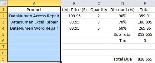
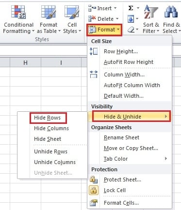
- Click the button “Format” in the ribbon.
- Then move your mouse to the option “Hide & Unhide”.
- Next, you will see a new menu. Here click the button “Hide Rows”. Thus, the target rows will hide.
And the thicker line here means that here are some hidden rows. In addition, you can also use the shortcut keys to hide rows. After you have selected the target area, press “Ctrl +9” and then those rows will hide.
As for columns, you can select the option “Hide Columns” in step 4. And the shortcut for hiding columns is “Ctrl +0”.
Show Rows or Columns (Method 1)
This part shows how to show rows or columns in corresponding with the first part.
- You need to first select certain areas. And here are several different conditions:
i. Select the two adjacent rows or any of two cells in the two adjacent rows of the hidden area.
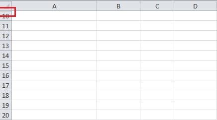
ii. If you have hidden the first row in the worksheet like this example, you can click the small area on the upper left part to select the whole worksheet.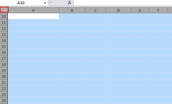
iv. Besides, you can also input a cell name of the target area into the “Name Box”. Thus, the cursor will position in the hidden area. You can see that the color of the corresponding column changes.
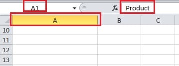
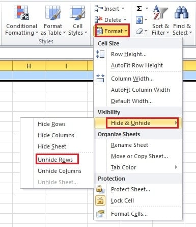
3. Then move your mouse to the option “Hide & Unhide”.
4. And in the menu, choose the “Unhide Rows”. Therefore, the hidden rows will appear again.
You can also use the shortcut key “Ctrl + Shift +9” to replace the step 3 – 4.
And for columns, you can choose “Unhide Columns” in step 4 and the shortcut is “Ctrl + Shift +0”.
Hide Rows or Columns (Method 2)
Except for the method above, you can also use this way.
- Select the whole area of the target area.

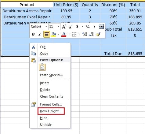
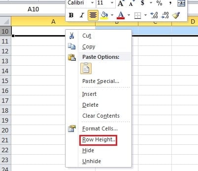
- And then right click.
- next in the menu, choose the option “Row Height”.
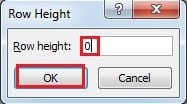
- And then set the height to “0”.
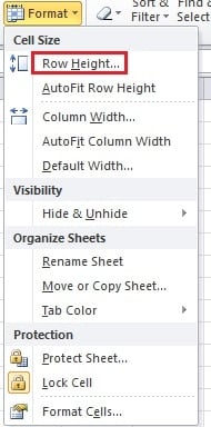
In addition, you can also set the row height in the “Format” menu.
- Last click “OK”. Thus, the rows will also hide.
And for column, you need to right click and select the option “Column Width”.
Show Rows or Columns (Method 2)
1. Here you should also select certain areas.
i. Select the two adjacent rows of the target area.
ii. If you hide the first rows in the area, you can select the whole worksheet.
iii. You can also first select the row next to the select area and then move upwards.
2. Then right click in the area.
3. In the new menu, click the “Row height”.
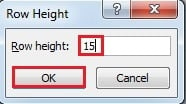
4. Then in the new window, input the height into the text box. The default height in Excel is 15. And you can also set according to your need.
5. Then click “OK”. Thus, the hidden rows will appear.
Excel Corruption can Harm your Data
If you suffer from an Excel corruption, you should be more careful about your Excel files. That is because your data in Excel will probably be destroyed. Thus, a third party tool can be a good helper. With this powerful tool, you can repair Excel quickly.
Author Introduction:
Anna Ma is a data recovery expert in DataNumen, Inc., which is the world leader in data recovery technologies, including word recovery and outlook repair software products. For more information visit www.datanumen.com
