4 Effective Methods to Zoom Your Excel Worksheet

The necessity to zoom Excel worksheet will come out at any time. Here we will introduce 4 effective methods to zoom Excel worksheet.

Sometimes you will zoom in an Excel worksheet to arrange its interface. And sometimes you will zoom out the worksheet to check certain values. Now we have 4 methods to fulfill this task.

Method 1: Use IntelliMouse

When you scroll the wheel of mouse, the worksheet will move upwards or move downwards. But here you can use the wheel to zoom the worksheet.

1. Click “File” in the ribbon.
2. Next click “Options”.
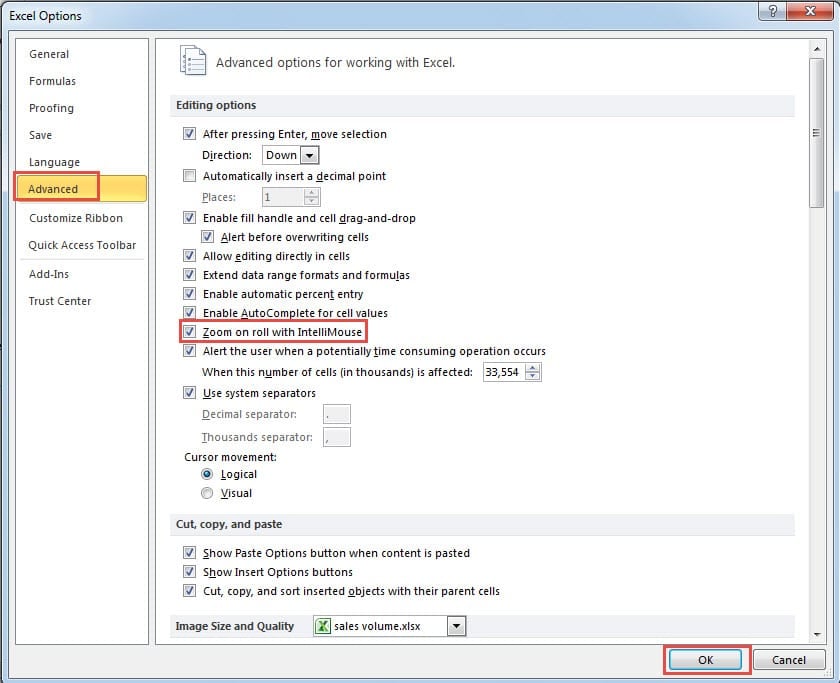
3. In the “Excel Options” window, click “Advanced”.
4. And then in the “Editing options”, check the option “Zoom on roll with IntelliMouse”.
5. After that, click “OK”.

Now, when you scroll the mouse wheel, the interface of worksheet will zoom in or zoom out. If you scroll down the wheel, the worksheet will zoom out. On the other hand, if you scroll up the wheel, the worksheet will zoom in. Besides, the zoom size of mouse wheel is 15%.

However, you may find that if you want to move the worksheet, you cannot use the mouse wheel any more. Here you can refer to our previous article 3 Practical Methods to Move around a Worksheet in Your Excel to move the worksheet. If you want to close this feature, you can also uncheck the option in step 4.

Method 2: Use Zoom Bar

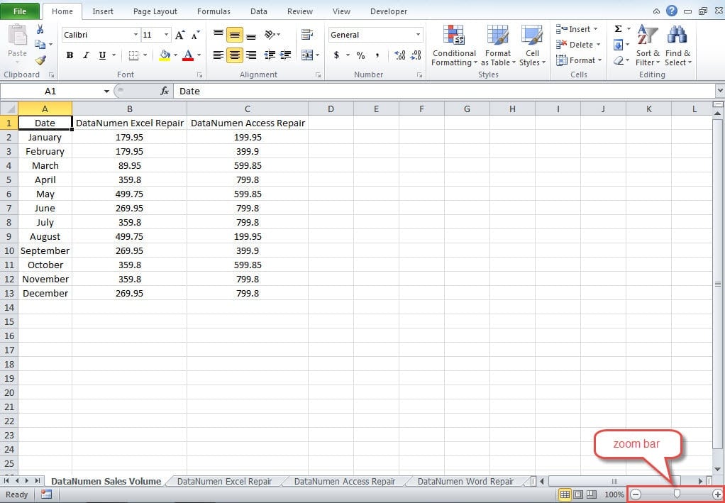
Instead of using the IntelliMouse, you can also use the zoom bar in the interface of worksheet. The zoom bar lies in the right bottom corner of the interface.

1. Here you can click the two buttons of “Zoom Out” or “Zoom In” to zoom the worksheet. The zoom size of the two buttons is 10% every time you click one of them.

2. Besides, you can also click on the bar directly. And the middle of the bar is 100%. When you click the right part of the bar, the worksheet will zoom in. And clicking the left part, the worksheet will zoom out.

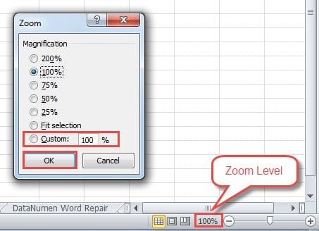
3. Except for click the buttons and the zoom bar, you can also click the “Zoom Level” to set the magnification directly.

When you click the “Zoom Level”, you will see the zoom window pop up. In this window, you can choose the pre-set magnification or input a customized number. Clicking “OK” and then the worksheet will change according to your setting.

Here if you choose the “Fit selection”, the size of the range that you select will be change to fit the screen. For example, in this image, we select the range A1:N13.

However, the screen is not big enough to show all the cells. When you choose “Fit selection”, the size of the selected range will change like the image below shows:

With the zoom level change, all the cells are able to be seen in the screen. So the next time if you want to show a range in one screen, you can also use this feature.

Method 3: Change in the Toolbar

You can also change the zoom level in the toolbar. Click the tab “View” in the ribbon. And then in the part of “Zoom”, you can see 3 options.

1. Click “Zoom” button in the area, you will see the “Zoom” window. This is the same as clicking the “Zoom Level” on the right bottom.
2. If you click “100%”, the zoom level of the worksheet will change into 100% immediately.
3. As for the “Zoom to selection”, it has the same effect as the function of the option “Fit selection” in the “Zoom window.

Thus, you can also choose to change the zoom level in the toolbar.

Method 4: Add Buttons in the Quick Access Toolbar

If you are used to adding buttons to the quick access toolbar, you can also add the zoom buttons into this area.

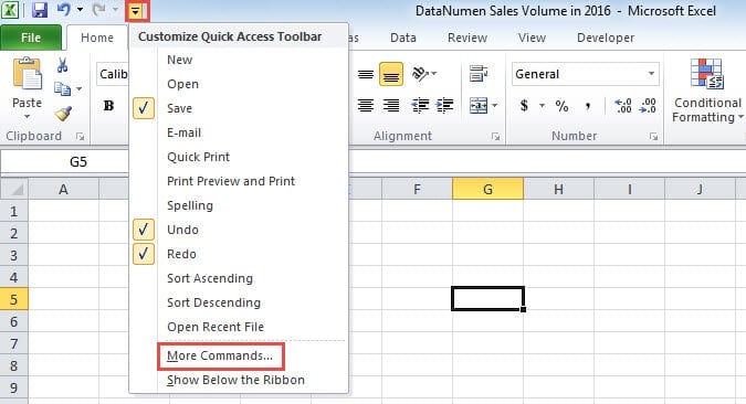
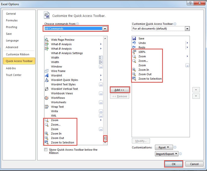
1. Click the small arrow in the quick access toolbar.
2. And then click “More Commands” in the drop-down menu.
3. In the “Choose commands from”, choose the option “All Commands”.
4. Now drag the scroll bar and find the buttons of zoom. There are 7 buttons about zoom feature in the options. The button “100%” lies in the beginning position. And other 6 buttons lie in the end of the list.
5. When you find one, click “Add” to add the button to the quick access toolbar.
6. After you add all the needed buttons in the bar, click “OK” in the window. Therefore, you have added the buttons in the quick access toolbar.

Although all the buttons serve for the function of zoom, they still have subtle difference with each other. And we will introduce then according to the order in the “Excel Options” window. You may refer to the image after step 5.

1. If you click the “100%” button, the zoom level of the worksheet will change back to 100%.
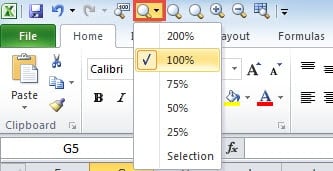
2. You will see a drop-down list if you click the first “Zoom” button.

There are 6 options in the menu. You can choose one of them. And the “Selection” is exactly the “Fit selection” in “Zoom” window.

3. The second zoom button will activate the “Zoom” window.
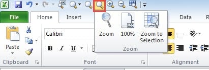
4. And then if you click the third zoom button, you will also see a menu pop up.

The three options in the menu are exactly the three options under the tab of “View”.

5. When you click “Zoom In”, the worksheet will zoom in. If the zoom level is less than 100%, the zoom level will first change into the number that is the closest to 25%, 50% or 75%. And then the level will add by 25% every time you click the button until it comes to 100%. And when the zoom level is between 100%-200%, when you click the button, the zoom level of the worksheet will become 200% directly. If the zoom level is greater than or equals to 200%, it will not become large when you click the button.
6. The “Zoon Out” button will reduce the zoom level of the worksheet. If the zoom level is larger than 200%, the level will change into 200% when you click the button. And then the level changes into 100% if you click it again. When the zoom level is between 100%-200%, the zoom level of the worksheet will become 100% when you click the button. As for the level that is smaller than 100, it will first change into the number that is nearest to 75%, 50% or 25%, and then reduce by 25% each time. When the level is 25%, the level will not reduce any more.
7. The last button “Zoom to Selection” is the same as option in the toolbar.

Among all those different buttons, you can leave the frequently used buttons in the toolbar.

Run a Specialized Recovery Tool if Excel Corrupts

Excel will sometimes corrupt unexpectedly. And at this time, your priority is to recover Excel. There are many different methods to finish this task. And among those methods, the most efficient way is using a specialized recovery tool. It is embed with the best technology in the world. Hence, you don’t need to worry about your Excel any more.

Author Introduction:

Anna Ma is a data recovery expert in DataNumen, Inc., which is the world leader in data recovery technologies, including word recovery and outlook repair software products. For more information visit www.datanumen.com