How to Use the Different Count Functions in Excel

Count functions are the most frequently used functions in Excel. In this article, we will discuss about the different 5 count functions in detail.

There are 5 variants of count functions: COUNT, COUNTA, COUNTBLANK, COUNTIF and COUNTIFS. Below we will talk about their usages in detail.

1.      COUNT

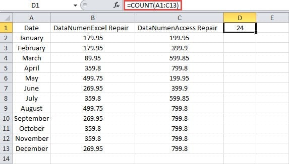
The COUNT function counts the numbers of cells that contains numbers in a designated range. Besides, it also counts the numbers in an array. And this range or array is the argument of the COUNT function. Now we want to count the cells in the range in the image below.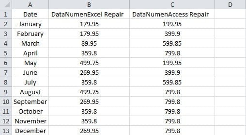

1. Click a blank cell where you need to show the result.
2. And then input this formula into the cell:

=COUNT(A1:C13)

We only input one argument into the formula. You can input up to 255 arguments into the formula.

3. And then press “Enter”. Thus, the result will appear in the cell immediately.

Actually there are 39 cells in the range. But other 15 cells contain contents instead of numbers. Therefore, the result is 24.

When it comes to multiple arguments, the COUNT function can also work perfectly. Now input the formula below into a blank cell:

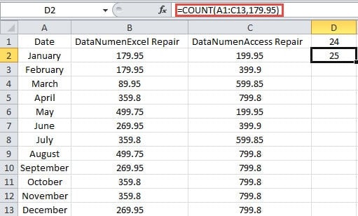
=COUNT(A1:C13,179.95)

And then you will get the result 25.

Some people may wonder that there are many cells that contain the number “179.95” in the range. Why the formula will get the result of “25”? Actually in the COUNT function, all the values in the formula are juxtaposed. Therefore, the number “179.95” has nothing to do with the range. As a result, the formula will add the numbers of the two values in the formula.

2.      COUNTA

The COUNTA function counts the numbers of nonblank cells in a range. As long as there are values in cells, including empty texts, this function will count those cells.

1. Click a blank cell.
2. Next input the formula into the cell:

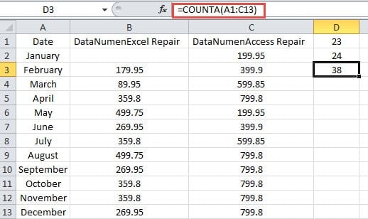
=COUNTA(A1:C13)

3. And then press the button “Enter”.

Here we delete the number in B2. Thus, you will see the result “38” instead of 39 in the cell.

Besides, this function can also add up to 255 arguments. Now if you input this formula into a cell:

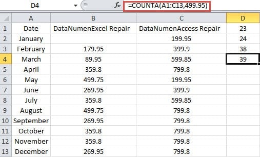
=COUNTA(A1:C13,499.95)

And then you will get the result “39”. This is the same as the COUNT function.

3.      COUNTABLANK

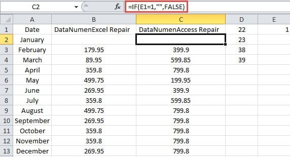
Different from the COUNTA function, the COUNTBLANK function counts the blank cells in a range. Here the blank cells also include cells with empty texts return by other formulas. In this example, we delete the number in cell B2. And in cell C2, we use an IF formula to return an empty value.

Now let’s see how the COUNTBLANK takes effect.

1. Click a blank cell.
2. And then input the formula into the cell:

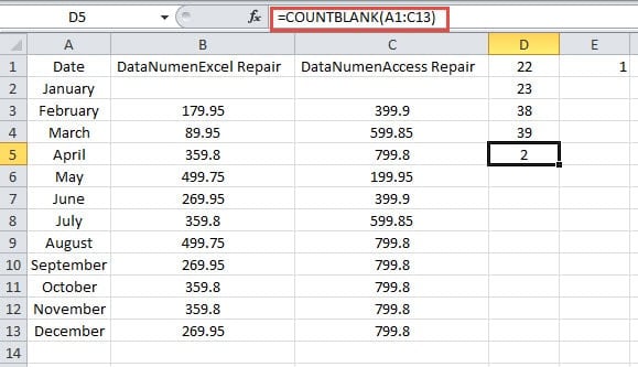
=COUNTBLANK(A1:C13)

3. Next press the button “Enter”. Thus, you will get the result.

The result means that even if there includes an empty text, this function will also count it. Cell D3 and D4 contain the COUNTA formulas. When the value is empty text in cell C2, the result of COUNTA functions don’t change. Hence, you need to be more careful about the empty text when using these two functions.

4.      COUNTIF

To count the number of cells meeting certain criterion, you can use COUNTIF function. We have already introduced the usage of this function in our previous article How to Count All Items Meeting a Condition via COUNTIF Function. And instead of the usage in the previous article, you can also use wildcard characters in formulas.

1. Click a blank cell in the worksheet.
2. And then input the formula into the cell:

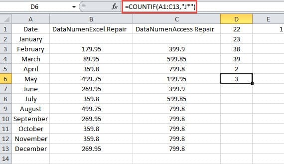
=COUNTIF(A1:C13,”J*”)

Here we want to search how many cells contain the values with the beginning of “J”. Therefore, the argument is “J*”in the formula.

3. Next press the button “Enter”. Now you can know that there are 3 cells contains the beginning of “J”.

5.      COUNTIFS

If you need to count cells meet multiple criteria, you need to use the COUNTIFS function. You can input multiple ranges and their corresponding criteria into the formula. Each range needs to have the same rows number and columns number. Otherwise this function cannot work. It may seem a little complex, and we will illustrate the usage through the example below.

1. Click a blank cell.
2. And then input the formula into the cell:

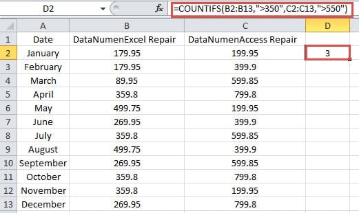
=COUNTIFS(B2:B13,”>350″,C2:C13,”>550″)

In this formula, we input two ranges into it.

3. Next, click the button “Enter”.

Here we input two ranges into the cell. We need to count the numbers across these two ranges with the given criteria. When the cells with the same relative position all meet the corresponding criteria, the formula will count 1.

The first cells in the two ranges are B2 and C2. But both of the values in the two cells don’t meet their corresponding criteria. Therefore, the formula will not add 1.

Let’s see the third cells B4 and C4. The number in B4 doesn’t meet the criterion while the number in C4 meets. Hence, this formula will also not add 1.

Now continue checking the forth cells B5 and C5. We find that both of the numbers meet the associated criteria. Thus, the formula will add 1 for these two cells.

According to the above analysis, you will have a better understanding of how the COUNTIFS function takes effect. Besides, you can add up to 127 ranges with their corresponding criteria.

Take Care of Your Formulas in Excel

Some formulas are very complex in Excel. Therefore, you need to pay more attention about them. Once you delete those complex formulas by accident, you need to review all the steps again to create it. And this is really very annoying. At this moment, you can use our potent tool to fix Excel. With this tool at hand, almost all the elements in Excel can be retrieved within minutes.

Author Introduction:

Anna Ma is a data recovery expert in DataNumen, Inc., which is the world leader in data recovery technologies, including word recovery and outlook repair software products. For more information visit www.datanumen.com