Sparkline – Mini Chart to Show Data Trends in Your Excel Worksheet

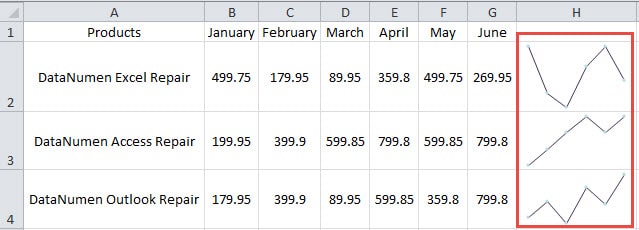
Chart in Excel will occupy a large area in Excel interface. Hence, you can use a tiny chart called sparkline to reflect the tendency of data instead.

You can create a sparkline in a cell, and this graphic will not take up a large area in the interface. For example, now you need to display the tendency of the sales volume, you can use the sparkline in this worksheet.

Add a Sparkline

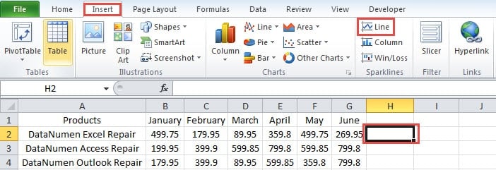
1. Click a cell where you want to put the sparkline.
2. Next click the tab “Insert” in the ribbon.
3. And then click the button “Line” in the area of “Sparklines” area in the ribbon.
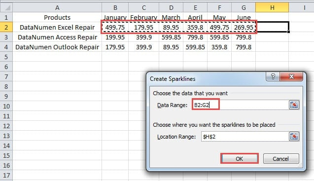
4. Next you will see the window “Create Sparklines”. Here input the data range into the textbox. You can either input the range manually or use the mouse to select the area.
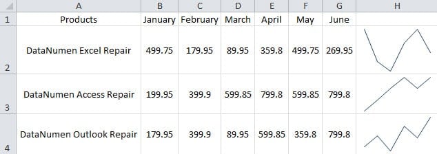
5. After that, click “OK” in the window. Therefore, the sparkline will appear in the cell.
6. Repeat the above steps and create sparklines for other products.in addition, you can also use the fill handle to add sparklines.

Modify the Sparkline

You will find that the sparkline is a little small. You can also modify them to make it better.

1. Change the cells width and height to make sparklines bigger in those cells.
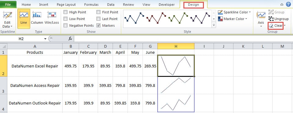
2. Select a cell with the line.
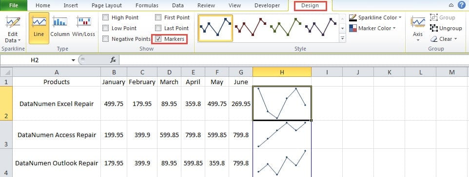
3. Click the tab “Design” in the ribbon.
4. And then check the option “Markers” in the toolbar. Thus, the markers will appear in the sparklines. Therefore, you can clearly see the tendency in those lines.
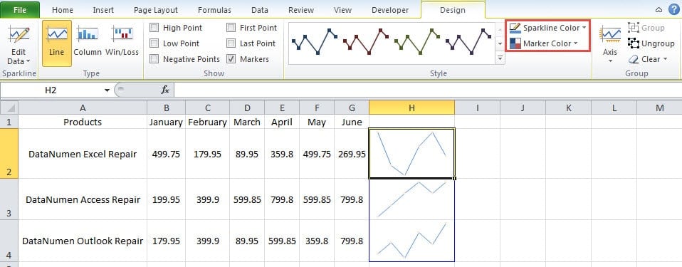
5. If you want to change the style, you can also set in the toolbar. In the style area in the toolbar, you can change the style of the sparklines. Besides, you can also change the color in the two options “Sparkline Color” and “Marker Color”.

Here in the image below, we also show a different style of those lines.

Delete Sparkline

You cannot delete the sparkline in Excel by pressing the button “Delete” on the keyboard. You need to use the feature in the toolbar in Excel.

1. Click the cell that you need to delete.
2. Next click the button “Design” in the ribbon.
3. And then click the button “Clear”.

Thus, the sparkline will be deleted from your worksheet.

Data Disaster will Compromise Your Excel Files

Sometimes you will meet with data disaster. And the result can be disastrous if you cannot handle it correctly. As a result, some of your Excel files will also be damaged. You can prepare an Excel recovery tool before you suffer from data disaster. Thus, whenever you find your Excel corrupts, you can fix it immediately.

Author Introduction:

Anna Ma is a data recovery expert in DataNumen, Inc., which is the world leader in data recovery technologies, including word recovery and outlook repair software products. For more information visit www.datanumen.com