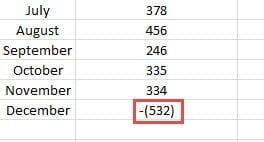
When you input numbers with parentheses into cells, they will change into negative numbers. And in this article, we will help you figure out this problem.
If you deal with Excel frequently, you may have already found this phenomenon. When you input parentheses for a number and then press “Enter”, the number in the cell will become a negative number immediately. The parentheses will be replaced by the minus sign “-“. To figure out the reason, you may continue reading this article.
An Example for this Phenomenon
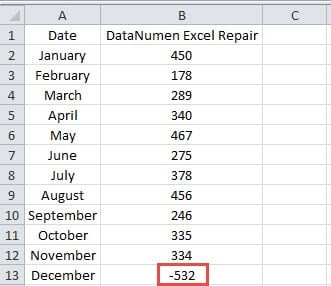
In this image below, we will input the sales volume of the month December. However, we don’t know the number yet. Therefore, we will input the estimated sales volume into the cell. To make a difference for this cell, we would like to add parentheses for this cell.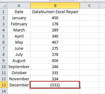
And then we press the button “Enter” on the keyboard. Instead of seeing the parentheses in the cell, you will see a minus sign appear.
And this will cause trouble to your work. But the reason is actually very simple. In Excel, numbers with parentheses are regarded as the other form of negative numbers. The cells format in Excel is “General” by default. When you input a number with parentheses, Excel will automatically treat this number as a negative number. And when you press the button “Enter” or click any other cell, the parentheses in a cell will automatically change into a minus sign. This is also a way of accounting bookkeeping.
The reason is very simple. But now if you still want to prevent the number from being taken as negative, you can follow the next part and see how to realize this task.
How to Solve this Phenomenon
Under the format of “General”, the form of the numbers will change. Therefore, here you can follow the steps below and learn to solve this problem.
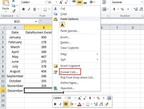
- Right click the target cell in the worksheet.
- And then choose the option “Format Cells” in the pop-up menu. In addition, you can also press the shortcut keys “Ctrl +1” on the keyboard to this step.
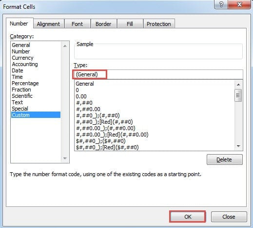
- And then in the “Format Cells” window, choose the category of “Custom”.
- After that, input this new type into the text box:
(General)
- Next click the button “OK” in the window.
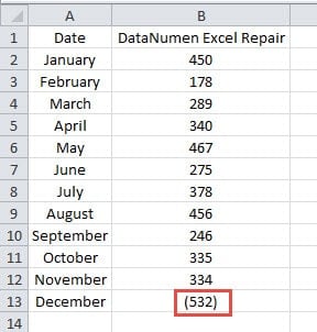
- Now you will come back to the worksheet. Here you can test your setting. Inputting a number into the target cell without parentheses.
- Next press the button “OK” on the keyboard or click any other cell in the worksheet. Then you will see that Excel will automatically add parentheses in this cell.
In this method, we don’t change the category into the “Number”. This is because in the “Number” category, the format with parentheses will still regard this number as negative numbers. And this will cause mistakes when you need to make calculation with this cell. Unless you need to show negative numbers with parentheses, you can use the “Number” category and choose the type with parentheses.
On the other hand, if you use the “General”, the format of negative number will still be clearly like the image below shows.
You will know immediately that this is a negative number. What’s more, you will never make mistakes when using this cell in calculation. Hence, you need to choose the most suitable category according to your actual need.
Prepare an Automated Backup Plan can Save You A Lot of Time
You may have already known the importance of backing up your Excel files. However, every time you back up your files, you will spend a lot of time. In order to solve this problem, you can prepare an automated backup plan. Thus, you never need to deliberately spend time and back up those Excel files. But sometimes even if you have backups of essential files, you still have the chance of losing data and information. Therefore, preparing an Excel recovery tool is rather important. Whenever you meet with problems, you can use this tool to repair Excel xlsx error.
Author Introduction:
Anna Ma is a data recovery expert in DataNumen, Inc., which is the world leader in data recovery technologies, including repair Word data damage and outlook repair software products. For more information visit www.datanumen.com
