How to Make Your Cell Values More Intuitive via Icon Sets in Excel

In Excel, you can use the icon sets to mark cells with different values. And in this article, we will talk about how to use this feature in Excel.

Icon sets is a very useful feature in Excel. It is also a small feature of the conditional formatting. Suppose now you need to mark cells for the sales volume in the worksheet.

Instead of ranking cells, now you can also use the different icons to mark different values in the cells, with icon sets, so to make these values more intuitive, as below:

And now follow the steps below to see how it works.

Add Icon Sets

1. Select the target range in the worksheet. Here we select the column B as an example.
2. Next click the button “Conditional Formatting” in the toolbar.
3. In the drop-down menu, move your cursor on the option “Icon Sets”.
4. And then in the submenu, choose one style that you prefer. Here we choose the directional style with three icons in the list.

Thus, the icon sets will appear in the range that you have selected.

Modify Icon Sets

The default style of the icon sets in Excel will rank the data automatically. Suppose now you need to rank the number “359.8” in the first level, you can also finish this task. Now you may follow the steps below and learn how to make this modification.

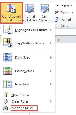
1. Click the button “Conditional Formatting” in the ribbon.
2. And then click the option “Manage Rules”.
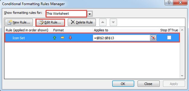
3. In the window of “Conditional Formatting Rules Manager”, choose the option “This Workbook” in the “Show formatting rules for”.
4. Now click the target rule that you need to modify.
5. And then click the button “Edit” rules in the window.
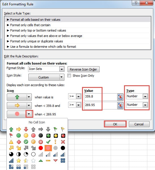
6. In the “Edit Formatting Rule” window, change the type into “Number”.
7. And then input the value into the two corresponding text boxes.
8. If you want to change the directional icon into other icons, you can also click the small arrow and choose one in the list.

In addition, except for the above three settings, you can also make other changes in this window according to your need. For example, you can change the rule type, the format style and others.

9. After you have finished the setting, click the button “OK” in the window.
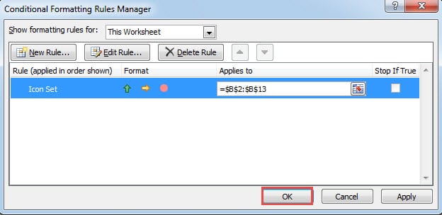
10. And then you will come back to the dialog “Conditional Formatting Rules Manager”. Here click “OK” in the window.

Thus, the new setting will immediately be applied in the range. You can see that the number “359.8” is also in the first level. And the icon of the last level is pink circle.

Form the above steps, you can see that setting the icon sets is very easy. And you can also apply this feature in your own worksheet.

Everyone Needs Excel Recovery Tool at Hand

Even though Excel does a lot of favor for us, it still has some flaws. Therefore, sometimes you will meet with Excel corruption. And once such an accident happens, you will certainly suffer a lot. Hence, you can prepare an Excel repair tool at hand. This tool is capable of fixing almost all the errors in Excel.

Author Introduction:

Anna Ma is a data recovery expert in DataNumen, Inc., which is the world leader in data recovery technologies, including word recovery and outlook repair software products. For more information visit www.datanumen.com