Pivot table can help us manage large data and information. In this article, we will introduce how to group or ungroup data in a pivot table.
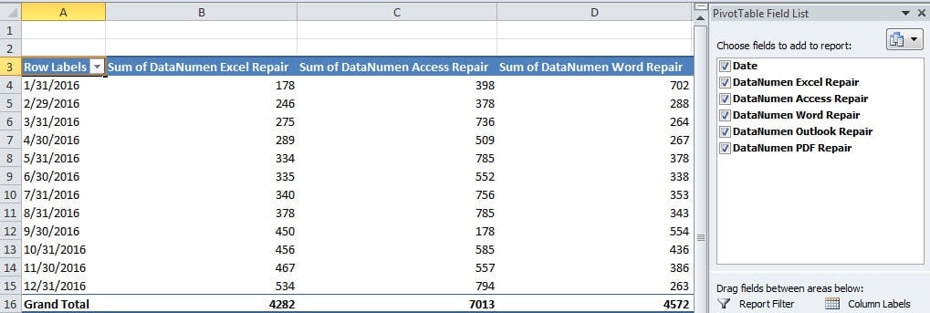
There are many useful features in pivot table. And those features make the pivot table a very useful tool for data analysis. The image below shows the pivot table in a worksheet.
The first column is the date of the range. By default, they will all be listed in the column A. But if you need to know the sales volume in a certain period, such as in a quarter, you need to have additional settings.
Group Data
In this part, we will show you how to group data in the pivot table.
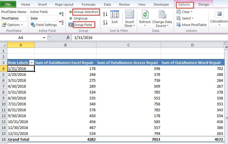
- Click a cell in the first column.
- And then click the tab “Options” in the ribbon.
- After that, click the button “Group Selection” or the button “Group Field” in the toolbar.
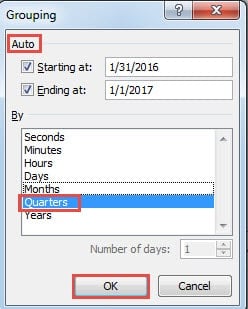
- And then you will see the “Grouping” window appear in the worksheet.
- In this window, the start date and the end date will appear automatically. If you only need to group a certain part, you can manually change the date.
- Next choose the criteria for the group. Here we will choose the “Quarters”.
- After that, click the button “OK” in the “Group” window. And then you will see the result in the pivot table.
The dates will change into the four quarters in the pivot table. And all the sales volumes will be calculated again. You can see that using this method is very convenient in analyzing data and information.
Group Selection
On the other hand, when you only need to know the sales volume of a certain quarter, the steps will be a little different.
- Click the three month in a quarter.
- And then click the tab “Options” in the ribbon.
- Next click the button “Group Selection”. At this time, you will also find that the button “Group Field” will be invalid. Because this time, you only select part of the field.
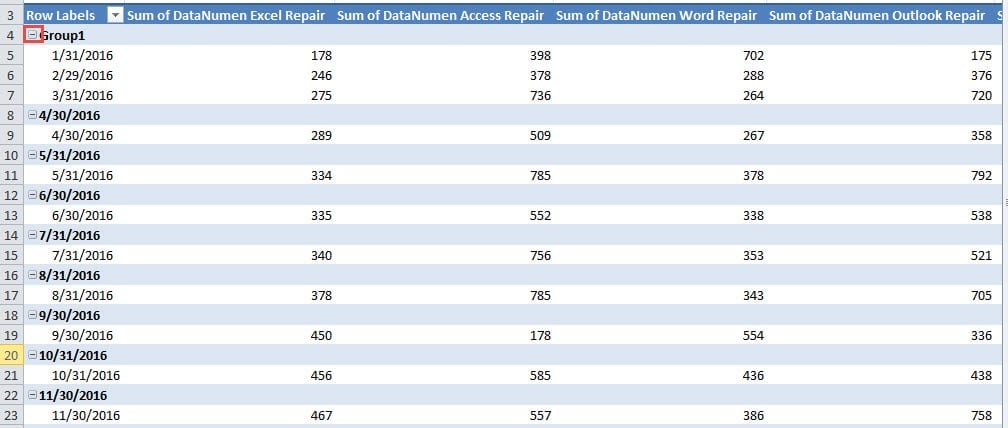
- Now the selected months will be grouped. There will be a “Group1” in the pivot table.
Click the minus symbol of the Gropu1, you will get the result.
When you need to group data in your pivot table, you can group the whole field or a part of it based on your needs.
Ungroup Data
When you finish the analysis, you will certainly need to ungroup your data and information. Follow the steps and see how to finish this task.
- Click the whole column in the pivot table. If you only group part of the range, click in the grouped part.
- And then still click the tab “Options” in the ribbon.
- After that, click the button “Ungroup”.
Therefore, the pivot table will change back. Ungrouping data is indeed very easy to finish.
Call a Data Recovery Company for Help
Whenever you meet with Excel corruption, you need to calm down. Most of the time, the lost data and information can be restored. You can call a data recovery company for help. Or you can also use an Excel recovery tool for help. This tool can repair corrupt Excel xls and fix other Excel errors easily. The data and information will always be safe with this tool at hand.
Author Introduction:
Anna Ma is a data recovery expert in DataNumen, Inc., which is the world leader in data recovery technologies, including repair corrupted doc and outlook repair software products. For more information visit www.datanumen.com


