Different cell colors can help you identify the values in cells. When you need to calculate values based on cell colors, you can use the 3 methods in this article.
In an Excel worksheet, you will certainly mark different colors for different cells. Most of the time, the same color will be in different cells in a range. The image below shows a worksheet with different cell colors.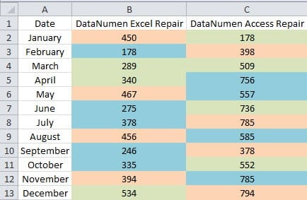
When you need to calculate the values by the cell color, you will find that it will be hard to select those cells. And now you can use the three methods in the following article to finish this task quickly.
Method 1: Use Sort Feature
When you need to calculate the values in a column or in a row, you can use this method.
- Select the target range in the worksheet.
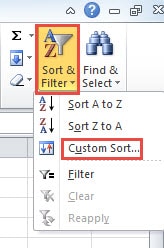
- And then click the button “Sort & Filter” in the toolbar.
- Next choose the option “Custom Sort” in the drop-down menu.
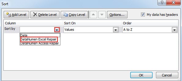
- In the “Sort” window, click the small arrow in the text box of “Sort by”.
- Next select the column that you need to sort.
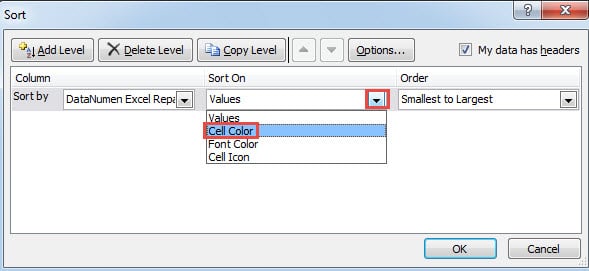
- And then click the arrow for the “Sort On”.
- After that, choose the option “Cell Color” in the list.
- Next you will see a new option in this window. Here click the small arrow for the “Order”.
- In the menu, choose the color that you need to calculate. Here we want to calculate the color of green, thus we choose the green color.
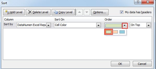
- After that, click the last small arrow.
- And then choose the “On Top” or the “On Bottom” according to your need. In this example, we will choose the “On Top”.
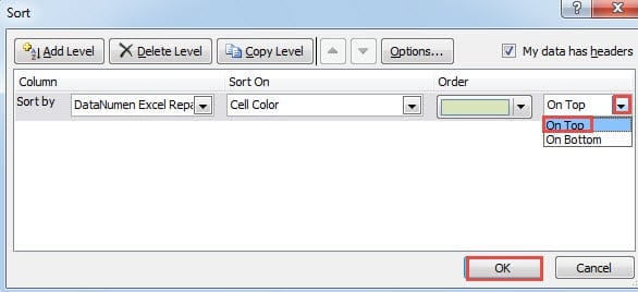
- When you finish the setting, click the button “OK” in this window.
And then you will come back to the worksheet, you will see that the values with green color will appear on the top of this column. Next you can calculate those values. In addition, it is very easy for you to choose the target range in this column.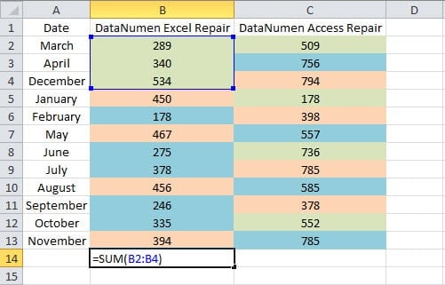
On the other hand, when you need to sort rows, you need to make addition setting.
- In the “Sort” window, click the button “Options”.
- And then choose the option “Sort left to right” in the “Sort Options” window.
- Next click the button “OK”.
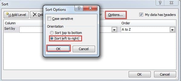
Thus, you can sort by rows in the target range. Other steps are the same as sort in columns. You can also have a try in your own worksheet.
Method 2: Apply Filter Feature
Except for the sort feature, here you can also apply the filter feature in Excel.
- Click a cell within the target range.
- And then click the button “Sort & Filter” in the toolbar.
- Next choose the option “Filter” in the menu.
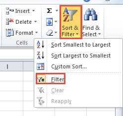
- Now you can see that the filter arrow will appear in the header row of the range. Click the arrow of the column that you need to filter.
- Next move your cursor to the option “Filter by Color”.
- And then in the sub menu, choose the color that you need to calculate.
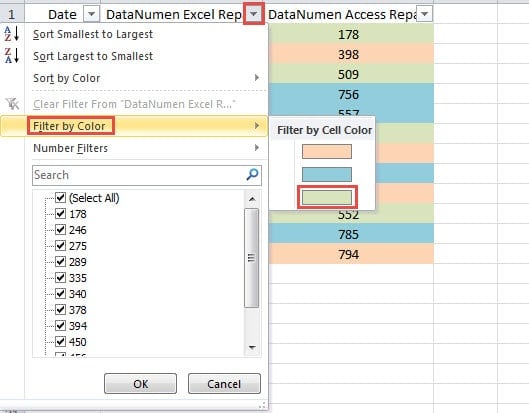
- Next you will find that only cells with the green color will appear in the worksheet.
When you need to calculate those cells, you can use the SUBTOTAL function. In this function, you need to choose the function that you need. And with SUBTOTAL function, you will get the result of corresponding numbers easily.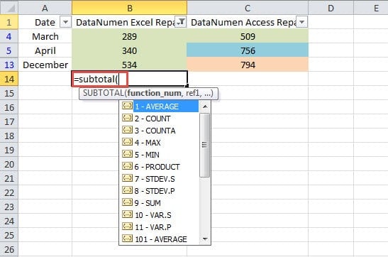
On the other hand, this method can only take effect on columns. If you need to calculate by rows, you need to use other methods.
Method 3: Use VBA Macros
The above two methods can calculate values in columns or rows. But when you need to calculate in a range that includes rows and columns, you need to use Excel macros.
- Press the button “Alt +F11” on the keyboard to open the Visual Basic editor.
- And then click the tab “Insert” in the toolbar.
- After that, choose the option “Module” in the sub menu.

- Now input the following VBA codes into this new module.
Function CalByColor(TarColor As Range, CalRange As Range)
  Dim TarCell As Range, CalCell As Double
    For Each TarCell In CalRange
      If TarCell.Interior.ColorIndex = TarColor.Interior.ColorIndex Then
        CalCell = WorksheetFunction.Sum(TarCell, CalCell)
      End If
    Next TarCell
  CalByColor = CalCell
End Function
Here we will use a user defined function to calculate the values. In this code, we will sum up the cells with the same value. When you need to do other calculations, such as count, average, you can also modify the codes according to your need.
- Now come back to the worksheet. When you need to calculate values of a certain color, you can first format a cell with this color in this worksheet.
- And then input the formula into another cell. Here we input this formula:
=CalByColor(E2,B2:C13)
- And then press the button “Enter” on the keyboard.
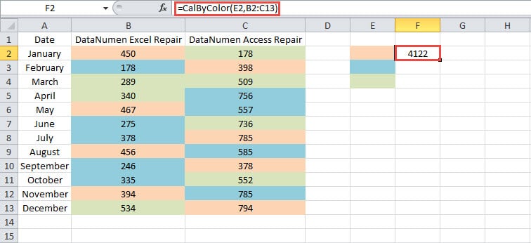
The result will immediately appear in the cell. If you only need to calculate cells in a column or a row, you can also change the range in this formula. As a result, using this user defined function is very easy for this task.
Make a Comparison between the Methods
From the above analysis, you can see that all the three methods are very useful. And in the table below, we have listed the advantaged and disadvantaged for you.
|
Comparison |
Use Sort Feature | Apply Filter Feature |
Use VBA Macros |
|
Advantages |
1. You can quickly sort the cells in a row or a column.
2. If you are not familiar with VBA codes, this method can be a good choice. |
1. By using the SUBTOTAL function, you can quickly calculate the target cells.
2. Compared with other two methods, this method is easy to manipulate and understand. |
1. You can use the user defined functions to finish the task easily.
2. This method will not be limited in a row or a column. |
|
Disadvantages |
1. If the target cells are in a range, you cannot use this method.
2. Every time you need to sort cells, you need to perform the steps again. |
1. This method can only be used in columns.
2. In using SUBTOTAL function, you may meet with error when choose the function and the reference. |
1. Using VBA codes will make things more complicated.
2. If you are not familiar with VBA macros, you will probably meet with errors when you need to modify the codes. |
Therefore, the next time if you need to choose a method, you can refer to this table. Choosing the most suitable method can help you finish your task quickly.
Standalone Recovery Tool can be Your First Choice
When you meet with Excel corruption, you will certainly need to repair it immediately. In order to repair you Excel quickly and easily, you can use a standalone recovery tool. You only need to install it in your computer, and it can repair Excel xlsx problem with a few clicks. Hence, even if you know nothing about data recovery, you can also recovery your damaged files.
Author Introduction:
Anna Ma is a data recovery expert in DataNumen, Inc., which is the world leader in data recovery technologies, including repair Word data error and outlook repair software products. For more information visit www.datanumen.com
