2 Methods to Make Column Chart More Intuitive by Changing Column Colors in Excel

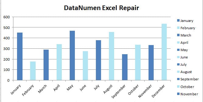
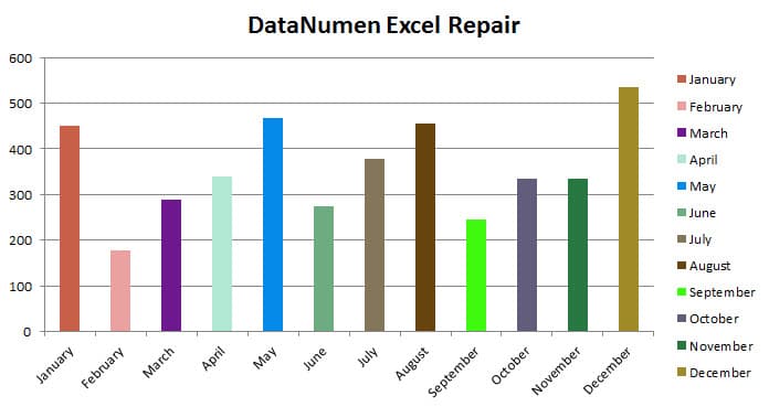
The column chart is frequently used in Excel. And to make it more intuitive, now you can use the 2 methods to change the column colors.

Column chart is the most ordinary chart in Excel. It is always used to display and analyze data and information. In the image below, you can see that there is an ordinary column chart in a worksheet.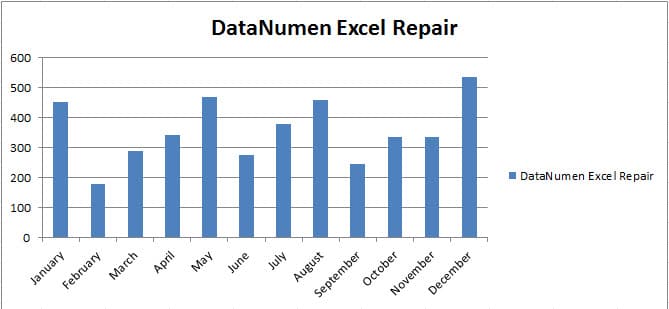

All the colors of those columns are the same. This is the default setting in Excel. And now you can also change the column colors to make your Excel more colorful.

Method 1: Change Colors Manually

Changing colors manually is the most ordinary method in Excel. Now follow the steps and see how it works.

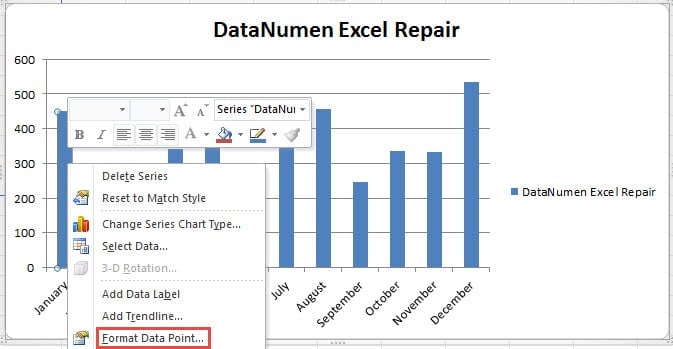
1. Click the column that you need to change the color. When you click it, you will see actually all the columns are selected.
2. And then click this column again. Thus, now you have only selected one column.
3. In the new menu, choose the option “Format Data Point”.
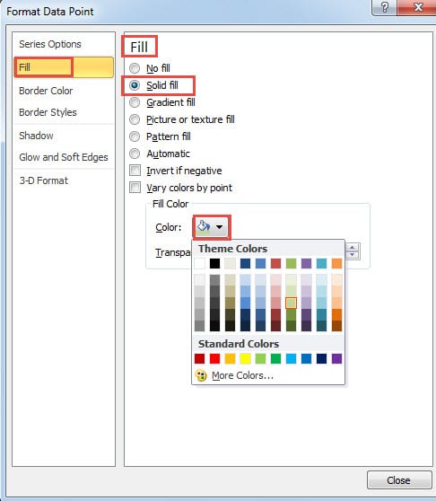
4. After that, you will see the “Format Data Point” window. In this window, click the option “Fill” on the left.
5. Next you will see many options for the fill. You can certainly choose to use other effects according to your preference. And here we will change the color, thus we choose the option “Solid Fill”.
6. Next click the button for “Color”.
7. In the drop-down list, choose a color that you need. If you are not satisfied with the theme color, you can also click the button “More Color” and set a special color.
8. Next change the “Transparency” if you need.
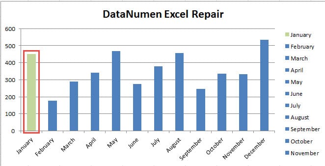
9. When you have finished all the settings, close this window. And you can find that in the chart, the color of this column has already changed.

On the other hand, the legend in this chart also changes accordingly.

Now you can repeat the above steps and change other column colors in this chart.

Method 2: Use VBA Macros

You will find that changing colors manually will cost you a lot of time and energy. Instead of changing manually, now you can also use the VBA macros in Excel to finish this task quickly. And below we have also provided two different macros to change column colors.

The first is changing colors every other column. Now follow the steps and see how to use this method.

1. Click the tab “Developer” in the ribbon.
2. And then click the button “Visual Basic”. Therefore, you have opened the Visual Basic editor. On the other hand, you can also press the shortcut keys “Alt + F11” on the keyboard to open the Visual Basic editor.
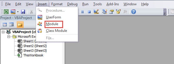
3. In this Visual Basic editor, click the tab “Insert” in the toolbar.
4. And then choose the option “Module” in the drop-down list. Thus, you will insert a new module in this editor.
5. In this step, copy the following VBA codes into this new module.

Sub OneColor()

    Dim i As Integer

    Sheets(1).ChartObjects("Chart 1").Activate

    For i = 2 To 13

        If i Mod 2 = 0 Then

            ActiveChart.SeriesCollection(1).Points(i).Format.Fill.ForeColor.RGB = RGB(176, 229, 242)

        End If

    Next i

End Sub

In this module, we will change the colors of every other column. In your actual worksheet, you need to change certain elements in this macro, such as the worksheet index, the chart index. Besides, you can also change the RGB parameters according to your preference.

6. Now click the button “Run Sub” in the toolbar or press the button “F5” on the keyboard to run this macro.
7. Now come back to the worksheet. You can see that the colors in this chart also change.

Hence, it is much easier for you to find certain column according to the different color.

And here comes the second macro. Instead of changing colors every other row, you can also change all the colors. And below are the steps of using the second macro.

1. Open the Visual Basic editor.
2. Insert a new module into the editor. And if you want to input this macro in the same module, you can just skip this step.
3. Now copy and paste the following codes into the module:

Sub ChangeAllColors()

    Dim i As Integer

    Sheets(1).ChartObjects("Chart 1").Activate

    For i = 1 To 12

        ActiveChart.SeriesCollection(1).Points(i).Format.Fill.ForeColor.RGB  = RGB(Int(Rnd() * 255), Int(Rnd() * 255), Int(Rnd() * 255))

    Next i

End Sub

In this macro, we will change all the colors in the chare. And here we use the function INT and RND to generate the random RGB parameters. Thus, the colors in the chart will change randomly. In your actual worksheet, you need to change the certain elements according to the actual need.

4. Now run this macro. And then in the worksheet, you can check the new result.

Whenever you run this macro, the colors in those columns of this chart will also change. You can see that now your worksheet is more colorful.

Choose Proper Backup Strategy

Many of you have already backed up your essential Excel files in a different storage device. But the backups will also corrupt due to various reasons. Therefore, you need to have a proper backup strategy. Incremental backups or full backups are the two different ways. And you can choose one method according to your need. Besides, checking the backup files periodically is also necessary. However, there still exist chances that you will suffer from Excel corruption. You may probably lose all your data and information. In order to repair Excel xls and fix other errors in Excel, now you can apply this potent third party tool. With the help of this tool, you can repair an even severely damaged Excel file in your computer.

Author Introduction:

Anna Ma is a data recovery expert in DataNumen, Inc., which is the world leader in data recovery technologies, including repair Word file and outlook repair software products. For more information visit www.datanumen.com