How to Use AND, OR and NOT Functions in Conditional Formulas

You can use conditional formulas in conditional formatting. And in this article, we will explore how to use AND, OR and NOT functions in the conditional formulas.

In conditional formatting, you can use the combination of IF function and AND, OR or Not functions. Besides, in conditional formulas, you can omit the IF in the formula. Below we will talk about the usage in detail.

AND Function

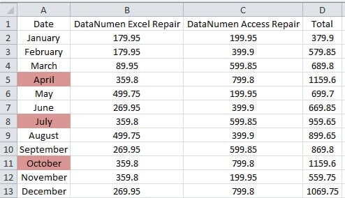
In the image below, we want to highlight the months with the criteria: the sales volume of “DataNumen Excel Repair” is greater than 350, and the sales volume of “DataNumen Access Repair” is greater than 400.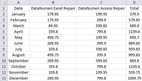

Therefore, here you need to use the AND function in the conditional formula.

1. Select the area that you need to highlight. And in this worksheet, we select the range A2:A13.
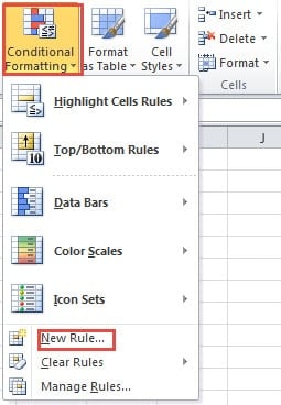
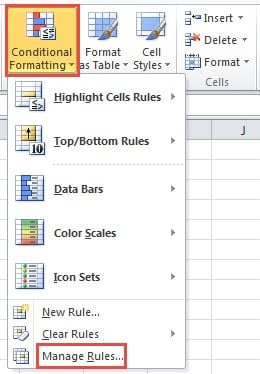
2. And then click the button “Conditional Formatting” in the toolbar.
3. Next choose the option “New Rule” in the drop-down list.
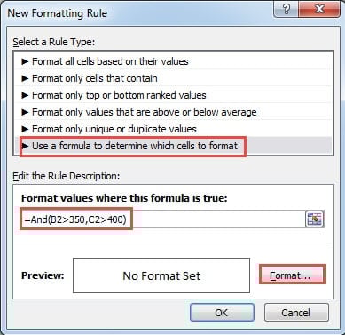
4. In the new rule window, choose the last option of formula in the list.
5. And then input this formula into the textbox:

=And(B2>350,C2>400)

Here you don’t need to input the IF function into the formula. If the condition is true, the corresponding cell will be highlighted. And in the formula, you only need to input the first cell of each range.

6. Next click the button “Format” in the window.
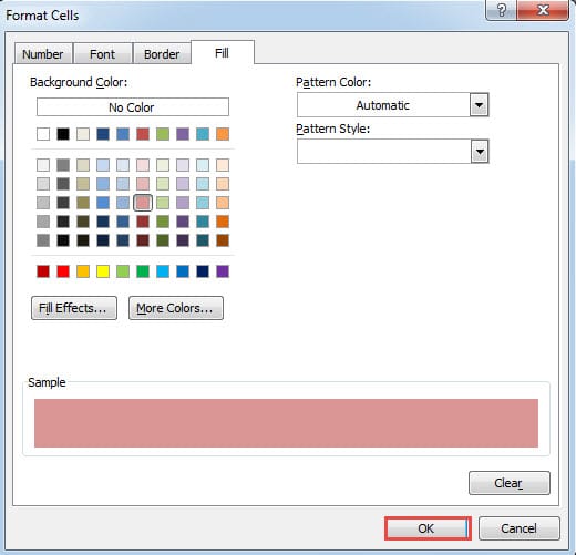
7. And then in the “Format Cells” window, set a different format for the cells that you want to highlight. Here we change the background color.
8. When you finished the setting, click “OK” in the window.
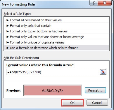
9. And then you will come back to the “New Formatting Rule” window. Here you can also preview the format. And click “OK” to confirm this setting.

Next you will come back to the interface of the worksheet. In the worksheet, cells that meet the criteria will be highlighted with the special format.

OR Function

Suppose you have changed the criteria into this criteria: the sales volume of “DataNumen Excel Repair” is greater than 350, or the sales volume of “DataNumen Access Repair” is greater than 400. Therefore, here you need to use the OR function in the conditional formula. If there is no conditional formatting in your worksheet, you can repeat the steps in the previous part. On the other hand, if there exist other conditional formatting in this range, you need to delete it and then add the new condition. Besides, you can also modify the existing criteria. And below we will show you how to modify the existing criteria based on the previous part.

1. Select the target range in the worksheet.
2. And then click the button “Conditional Formatting” in the toolbar.
3. Next choose the option “Manage Rules” in the list.
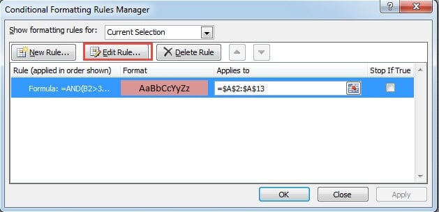
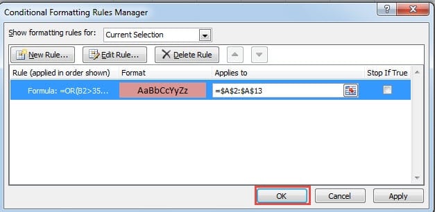
4. In the “Conditional Formatting Rules Manager” window, double click the existing rule. Or you can also click the rule and then click the button “Edit Rule”.
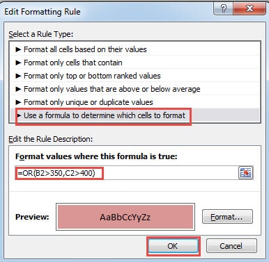
5. In the “Edit Formatting Rule” window, make sure that the rule type is “Use a formula to determine which cell to format”.
6. And then input the formula into the text box:

=OR(B2>350,C2>400)

Here you only need to change the AND into the function OR.

7. Change the format if you need.
8. And then click the button “OK” in the window.
9. In the “Conditional Formatting Rules Manager” window, click the button “OK” again.

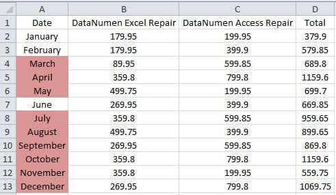
Thus, you can see the new result in the worksheet.

NOT Function

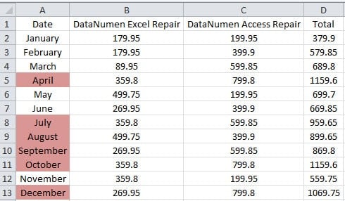
In this part, we will talk about the NOT function. Here we also change the criterion. We need to highlight the months whose total sales volume is not less than 700. You can either delete the existing conditional formatting and create a new one or edit the existing criteria. Still we will modify the existing criteria.

1. Repeat the first 5 steps in the OR Function
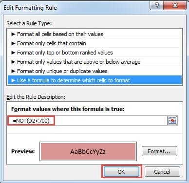
2. Now input this formula into the text box:

=NOT(D2<700)

3. You can click the “Format” if you still need to change the format.
4. And then click “OK” in the window.
5. Next click “OK” in the “Conditional Formatting Rules Manager” window.

Therefore, you can also see the new result in the worksheet.

From the above analysis, you can see that using AND, OR and NOT functions in conditional formulas is very easy. The only thing you need to pay attention is that don’t leave two different conditional formatting in the same range. Otherwise you will be mixed by the different results. And in your actual worksheet, combining those functions in Excel can help you a lot.

Excel Damage will Make Your Life Miserable

Nowadays there exist many reasons that will cause damage to your Excel files. Some common reasons include human mistakes, virus, malware, hardware failure, power failure and others. To be honest, some of the reasons are unavoidable. Therefore, you need to prepare for repairing Excel files. Now, you can use a third party tool for help. This tool is specially designed to repair xls data error. Almost all the errors can be handled easily with this tool.

Author Introduction:

Anna Ma is a data recovery expert in DataNumen, Inc., which is the world leader in data recovery technologies, including repair doc data corruption and outlook repair software products. For more information visit www.datanumen.com