There are many table styles in your Excel worksheet. But instead of using the pre-defined styles, you can also create your own custom table style in Excel.
When you create a new table in the worksheet, you will see the default table style in the range. With different colors in adjacent rows, you can check values more convenient.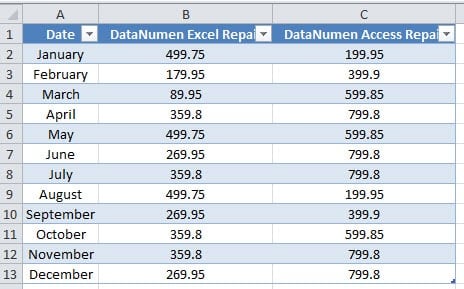
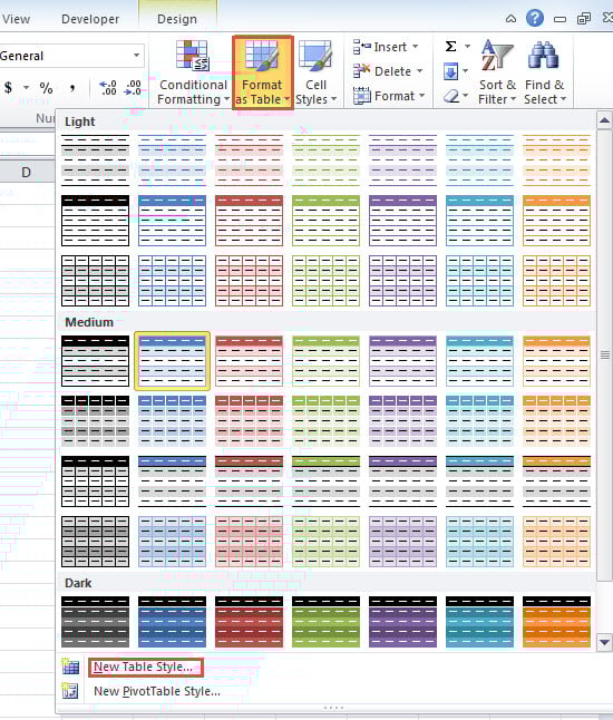
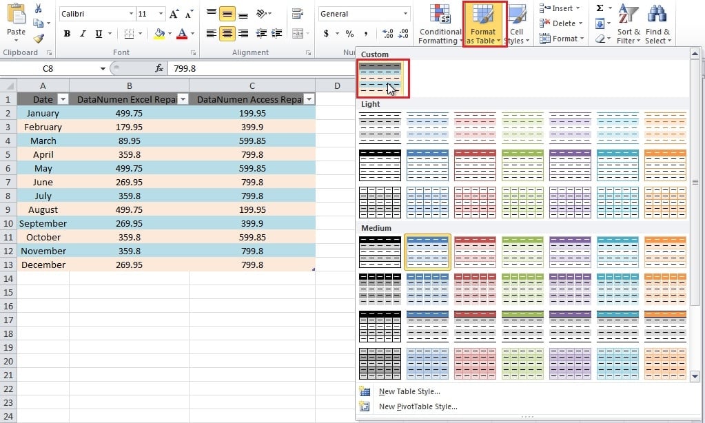
But if you are bored with the default table style, you can also change it. You can click the button “Format as Table” and open the style list. In the image below, you can see that there are many table styles available. Choose one of them according to your need.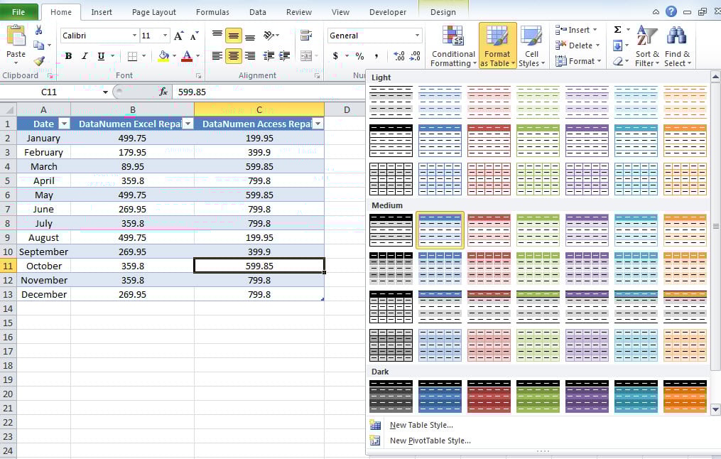
However, what if you are still not satisfied with all of those default styles in Excel? Now follow the steps below and create your own custom table style.
Create a Custom Table Style
- Click the button “Format as Table” in the toolbar.
- And then click the button “New Table Style” in the list.
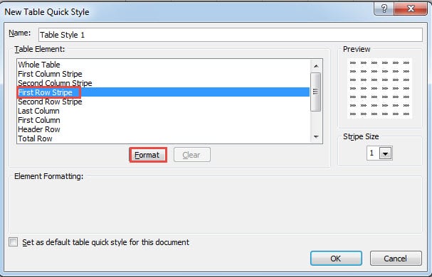
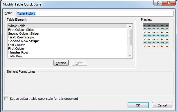
- Now in the new window, you can customize the style. Change the name if you need. And we will keep the default name in this example.
- Here we click the option “First Row Stripe” in the “Table Element”.
- Next click the button “Format”.
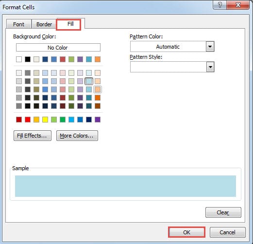
- In the “Format Cells” window, set the format for the first row in the range. Here we will fill the row with a specific color.
- When you finish the setting, click the button “OK”. And then you will come back to the “New Table Quick Style” window.
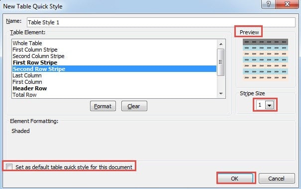
- Now continue setting format for other table elements. You can also see the preview the result in the “Preview” area.
- There are some stripes in table elements. And you can change the stripe size in this window according to your need.
- Besides, there is also an option “Set as default table quick style for this document” in the bottom. You can choose to check this option according to your need.
- After that, click the button “OK” in the window. Thus, you have created a new custom table style.
- Now you can apply the style in your table. Click a cell within the table range.
- And then click the button “Format as Table” in the toolbar.
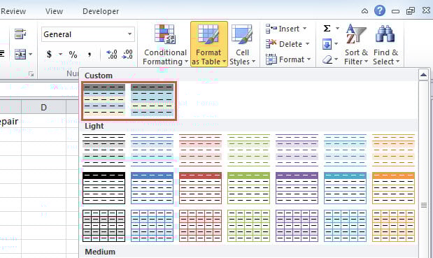
- Now you can see the custom table style in the list. When you move your mouse on this style, you can preview the result in the worksheet. And if you need to apply this style, just click it.
Therefore, you have now applied the new style in the table. But remember that you can only use this style in the current workbook. In other workbook, you cannot see this option in the list.
When you need to modify the style or delete, you may follow the steps below.
Modify Table Style.
- Still click the button “Format as Table” in the toolbar.
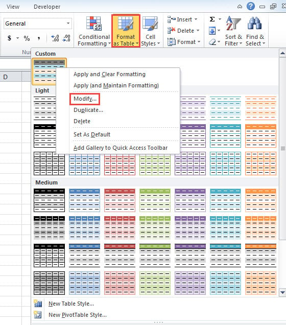
- In this step, right click the custom table style that you need to modify.
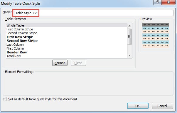
- And then in the menu, choose the option “Modify”. Thus, you will open the “Modify Table Quick Style” again.
Therefore, you can modify the settings in the window again.
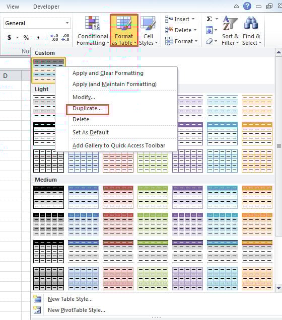
But on the other hand, you will sometimes need to keep the original style. Hence you can choose the option “Duplicate” in step 2.
Now in the window, you will see that Excel will automatically add “2” into the name to show the difference.
When you finish the setting and click “OK” in the window, you will find that there are two table styles in the list. The original one is still exist in the list.
Delete Table Style
If you will never use the custom table style, this style will only take up the memory in this file. Thus, you can also delete it from this workbook.
- Click the button “Format as Table” in the toolbar.
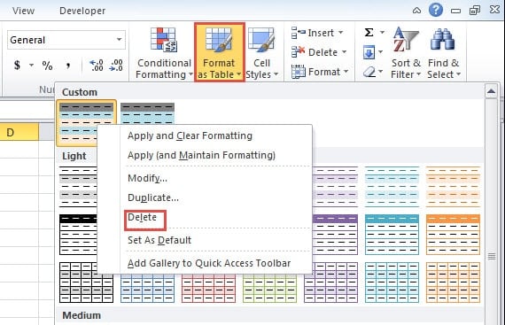
- Now right click the style that you don’t need.
- After that, choose the option “Delete” in the sub menu.
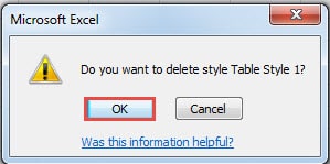
- And then you will see this information like the image below shows.
Here click “OK” to confirm the deletion. Thus, the table style has been removed from your Excel workbook. If there is a table that uses this custom table style, you will also find that the style of the table will turn back to the default style. And you cannot use this table style any more.
Retrieve Your Custom Table Style
Instead of deleting the table manually, some other reasons can also destroy your custom table style. Actually at this moment, you don’t want to lose your table style. However, once those accidents happen, you will lose access to those styles. Besides, small errors in Excel will sometimes result in severe result. Hence, you need to pay high attention to your Excel files. In addition, you can also prepare a potent repair tool at hand. Therefore, you can repair xlsx data problem quickly with this tool once accidents happen. And all the missing table styles can also be retrieved easily by this software.
Author Introduction:
Anna Ma is a data recovery expert in DataNumen, Inc., which is the world leader in data recovery technologies, including repair docx file damage and outlook repair software products. For more information visit www.datanumen.com
