
1. Introduction
Managing complex Excel workbooks with numerous worksheets can become overwhelming, especially when you need to track, reference, or organize multiple sheets efficiently. The ability to list sheet names in Excel becomes an essential skill for any professional dealing with large-scale spreadsheet operations, from financial models to comprehensive data analysis workbooks.
When faced with creating an Excel list of sheet names, many users find themselves manually scrolling through worksheet tabs, which becomes impractical for workbooks containing substantial numbers of sheets. The methods outlined in this guide will help you get all sheet names in Excel regardless of workbook complexity, offering solutions from simple manual approaches to sophisticated automation scripts for any Excel worksheet inventory requirement.
2. Method 1: Get List Manually
The manual approach represents the most straightforward method to Excel get all sheet names, requiring no advanced Excel knowledge or formula creation. This technique works particularly well for smaller workbooks where the total number of worksheets remains manageable, typically fewer than twenty sheets.
- First off, open the specific Excel workbook containing the worksheets you want to catalog.
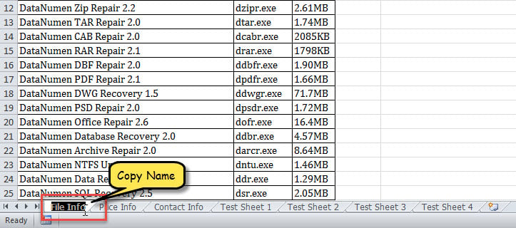
- Then, double click on a sheet’s name in the sheet list at the bottom of the Excel interface. This action will select the entire sheet name text, highlighting it for easy copying.
- Next, press “Ctrl + C” to copy the selected name to your clipboard for transfer to your documentation file.

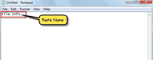
- Later, create a text file, Word document, or new Excel worksheet where you want to maintain your comprehensive sheet name inventory.
- Then, press “Ctrl + V” to paste the copied sheet name into your chosen documentation format.

- Now, in this systematic way, you can copy each sheet’s name to your documentation file one by one, building a complete inventory of all worksheets in your workbook.
3. Method 2: List with Formula
The formula-based approach to Excel list all sheet names leverages Excel’s built-in functions to automatically generate a comprehensive worksheet inventory. This method combines the power of Excel’s GET.WORKBOOK function with dynamic indexing capabilities, creating a self-updating list that reflects the current state of your workbook structure.
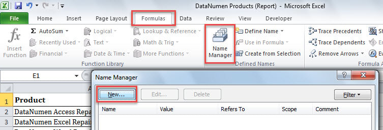
- At the outset, navigate to the “Formulas” tab in Excel’s ribbon interface and click the “Name Manager” button to access Excel’s name definition capabilities.
- Next, in the popup Name Manager window, click “New” to create a custom named range that will contain your worksheet listing formula.

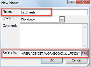
- In the subsequent “New Name” dialog box, enter “ListSheets” in the “Name” field to create a memorable reference for your worksheet listing formula.
- Later, in the “Refers to” field, carefully input the following specialized formula that will extract worksheet names from your workbook structure:
=REPLACE(GET.WORKBOOK(1),1,FIND("]",GET.WORKBOOK(1)),"")
- After that, click “OK” and “Close” to save this custom formula definition, making it available for use throughout your workbook.
- Next, create a new worksheet in the current workbook specifically for displaying your comprehensive sheet name inventory.
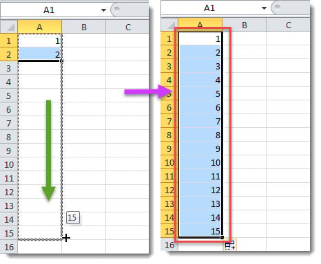
- Then, enter “1” in Cell A1 and “2” in Cell A2 to establish the indexing sequence that will reference each worksheet in your workbook.
- Afterwards, select both cells (A1 and A2) and drag them down to automatically input sequential numbers (3, 4, 5, etc.) in Column A, creating enough index numbers to cover all worksheets in your workbook.

- Later, put the following INDEX formula in Cell B1 to begin extracting worksheet names using your previously defined “ListSheets” name:
=INDEX(ListSheets,A1)
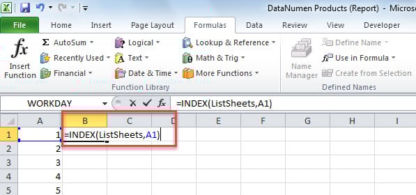
- At once, the first sheet name will appear in Cell B1, demonstrating that your formula configuration is working correctly.
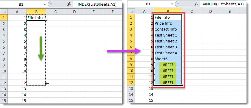
- Finally, copy this INDEX formula down the entire Column B until you encounter the “#REF!” error, which indicates you’ve reached the end of available worksheets in your workbook.

4. Method 3: List via Excel VBA
The VBA (Visual Basic for Applications) approach represents the most sophisticated and automated method to list all sheet names in Excel. This programming-based solution creates a completely automated worksheet inventory system that generates a new workbook containing a professionally formatted list of all worksheet names.
- For a start, trigger Excel VBA editor by pressing Alt + F11 or following the detailed instructions in Excel’s Developer tab to access the Visual Basic development environment.
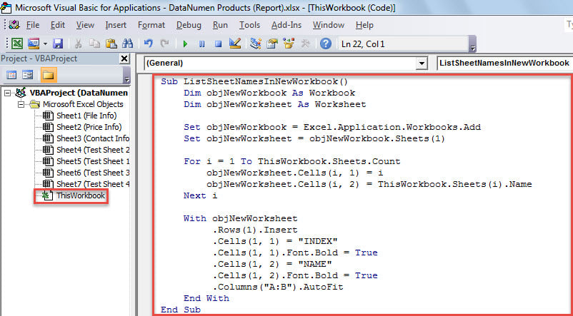
- Then, insert a new module into your VBA project and paste the following comprehensive code that will automatically extract and format all worksheet names from your current workbook:
Sub ListSheetNamesInNewWorkbook()
    Dim objNewWorkbook As Workbook
    Dim objNewWorksheet As Worksheet

    Set objNewWorkbook = Excel.Application.Workbooks.Add
    Set objNewWorksheet = objNewWorkbook.Sheets(1)

    For i = 1 To ThisWorkbook.Sheets.Count
        objNewWorksheet.Cells(i, 1) = i
        objNewWorksheet.Cells(i, 2) = ThisWorkbook.Sheets(i).Name
    Next i

    With objNewWorksheet
         .Rows(1).Insert
         .Cells(1, 1) = "INDEX"
         .Cells(1, 1).Font.Bold = True
         .Cells(1, 2) = "NAME"
         .Cells(1, 2).Font.Bold = True
         .Columns("A:B").AutoFit
    End With
End Sub
- Later, press “F5” key or click the “Run” button to execute this macro immediately, triggering the automated worksheet name extraction and formatting process.
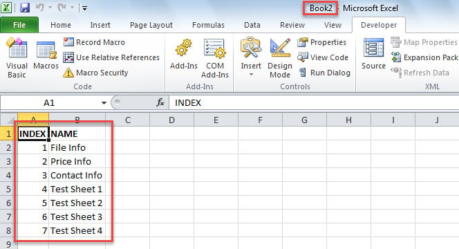
- At once, a new Excel workbook will appear on your screen, containing a professionally formatted list of all worksheet names from your source workbook, complete with index numbers and bolded headers for easy reference.

5. Method 4: Power Query Approach
Power Query offers a modern data connection method to Excel list all sheet names efficiently. This approach works exceptionally well for analyzing multiple workbooks simultaneously and provides a user-friendly interface for data extraction without requiring programming knowledge.
- Go to Data -> Get Data -> From File -> From Workbook.
- Select your current workbook file in the file browser dialog.
- Power Query Navigator will display all available sheet names automatically.
- Select the sheets you want to include and click Load to create a comprehensive list.
- The resulting table will contain all sheet names and can be refreshed when worksheet structures change.
6. Method 5: Dynamic Array Formula (Excel 365)
Excel 365 users can leverage dynamic arrays to get all sheet names in Excel using advanced formula combinations. This method creates automatically updating arrays that reflect current workbook structure.
- Enter the following formula in any empty cell:
=INDIRECT("Sheet"&SEQUENCE(COUNTA(GET.WORKBOOK(1)),,1)&"!A1")
- Press Enter to execute the dynamic array formula.
- The formula will create a spilling array showing references to all sheets in your workbook.
7. Method 6: Power Automate Integration
Microsoft Power Automate provides enterprise-level automation for Excel list of sheet names across multiple workbooks. This method excels in organizational environments requiring regular workbook analysis and reporting.
- Access Power Automate through your Microsoft 365 portal.
- Create a new flow using the Excel connector.
- Use the List worksheets action to extract sheet names programmatically.
- Configure output destinations such as SharePoint lists, emails, or other business applications.
- Set up automated triggers for regular worksheet inventory updates.
8. Method 7: Office Scripts (Modern Excel)
Office Scripts provide a TypeScript-based alternative to VBA for modern Excel environments. This method works exclusively with Excel Online and offers cloud-native automation capabilities to list all sheet names in Excel.
- Open your workbook in Excel Online.
- Navigate to Automate -> Script Editor.
- Create a new script with the following TypeScript code:
function main(workbook: ExcelScript.Workbook) {
  let sheets = workbook.getWorksheets();
  let sheetNames = sheets.map(sheet => sheet.getName());
  console.log(sheetNames);
}
- Click Run to execute the script and display sheet names in the console.
- Modify the script to output results to worksheet cells if needed.
9. Method 8: Python Programming
Python scripting provides powerful automation capabilities to Excel get all sheet names from single or multiple workbooks. This method offers excellent batch processing capabilities for large-scale worksheet analysis.
- Install required Python libraries using: pip install openpyxl pandas
- Create a Python script with the following code:
import openpyxl
workbook = openpyxl.load_workbook('your_file.xlsx')
sheet_names = workbook.sheetnames
for name in sheet_names:
    print(name)
- Replace ‘your_file.xlsx’ with your actual file path.
- Run the script using python script_name.py in your command prompt.
10. Method 9: Excel Add-ins
Third-party Excel add-ins provide specialized tools to list sheet names in Excel with enhanced functionality and user-friendly interfaces. Popular add-ins include comprehensive workbook analysis features.
- Install reputable add-ins like Kutools for Excel or ASAP Utilities.
- Access the add-in’s Workbook or Navigation tools from the ribbon.
- Use the List Sheet Names or Workbook Analysis feature.
- Configure output format and destination for the generated sheet list.
- Export or save the results according to your documentation requirements.
11. Method 10: XML File Analysis
Excel workbooks (.xlsx files) are ZIP archives containing XML structure data. This technical method allows direct extraction of sheet names without opening Excel, useful for automated file analysis scenarios.
- Create a copy of your Excel file and change the extension from .xlsx to .zip.
- Extract the ZIP archive using any file compression tool.
- Navigate to the xl folder and open workbook.xml in a text editor.
- Locate <sheet> elements containing name=”” attributes.
- Extract the sheet names from the XML structure manually or using text processing tools.
12. Method 11: Hyperlink Reference Method
The HYPERLINK function provides an indirect way to Excel list all sheet names by creating clickable links to each worksheet. This method generates a functional navigation system while documenting sheet names.
- In a new worksheet, start entering a HYPERLINK formula: =HYPERLINK(“#”
- When you type the sheet reference, Excel will display available sheet names in a dropdown.
- Complete the formula: =HYPERLINK(“#Sheet1!A1″,”Sheet1”)
- Create similar formulas for each sheet, building a comprehensive navigation list.
- Copy the sheet names from the formula text to create your documentation list.
13. Method 12: PowerShell Automation
Windows PowerShell with Excel COM objects enables system-level automation to get all sheet names in Excel. This method provides robust scripting capabilities for Windows environments requiring batch processing.
- Open PowerShell as Administrator.
- Execute the following PowerShell commands:
$excel = New-Object -ComObject Excel.Application
$workbook = $excel.Workbooks.Open("C:\path\to\your\file.xlsx")
$workbook.Sheets | ForEach-Object { $_.Name }
$workbook.Close()
$excel.Quit()
- Replace the file path with your actual Excel file location.
- The script will output all sheet names to the PowerShell console.
- Pipe the output to a text file using | Out-File sheet_names.txt if needed.
14. Comparison
Understanding the strengths and limitations of each method helps you choose the most appropriate approach for your specific worksheet documentation requirements. The following comparison evaluates each technique across multiple criteria including ease of use, efficiency, scalability, and practical applications in different work environments.
| Method | Advantages | Disadvantages |
| Manual | Easy to operate, requires no technical knowledge, works across all Excel versions | Time-consuming for large workbooks, prone to human error |
| Formula | Automatically updates when sheets change, creates permanent documentation | Requires formula knowledge, may not work in all Excel versions |
| VBA | Quick and convenient, highly customizable, professional output | Requires macro security settings, needs VBA knowledge for customization |
| Power Query | User-friendly interface, works with multiple workbooks, refreshable | Modern Excel versions only, requires data connection knowledge |
| Dynamic Array | Modern formula approach, automatically updating, compact solution | Excel 365 only, complex formula syntax |
| Power Automate | Enterprise automation, integrates with business systems, scheduled execution | Requires Microsoft 365 subscription, complex setup for beginners |
| Office Scripts | Modern cloud-based automation, TypeScript syntax, shareable | Excel Online only, requires programming knowledge |
| Python | Powerful batch processing, cross-platform, extensive libraries | Requires Python installation and programming skills |
| Add-ins | User-friendly, feature-rich, professional tools | Additional cost, potential compatibility issues, external dependency |
| XML Analysis | Works without Excel, technical insight into file structure | Complex technical process, requires file format knowledge |
| Hyperlink | Creates navigation system, visual sheet discovery | Indirect method, manual formula creation required |
| PowerShell | System-level automation, batch processing capabilities | Windows only, requires scripting knowledge, COM object dependencies |
Each method serves different user needs and organizational requirements. The manual approach works best for occasional use with smaller workbooks, while formula and VBA methods provide ongoing documentation capabilities. Power Query and Power Automate excel in business environments requiring regular analysis, while programming approaches like Python and PowerShell offer maximum flexibility for advanced users. Add-ins provide user-friendly solutions for frequent worksheet management tasks. For optimal results with any method, ensure your Excel workbooks are functioning correctly – corrupted files should be restored using Excel file repair software before attempting sheet name extraction.
Regardless of which method you choose to Excel list all sheet names, having a systematic approach to worksheet documentation significantly improves workbook management, collaboration efficiency, and overall data organization standards within your projects or organization. From simple manual copying to sophisticated automation scripts, these twelve approaches provide comprehensive solutions for any Excel worksheet inventory requirement.
Reference
- Microsoft Support. (2024). SHEETS function. Microsoft Excel Help & Training.
- Microsoft Support. (2024). Macro to loop through all worksheets in a workbook. Microsoft Excel VBA Documentation.
- Microsoft Learn. (2024). Excel.Workbook function. Power Query M formula language reference.
- Microsoft Support. (2024). HYPERLINK function. Microsoft Excel Function Reference.
- Microsoft Support. (2024). Create or edit a hyperlink. Microsoft Excel Help & Training.
- Microsoft Support. (2024). Overview of formulas in Excel. Microsoft Excel Formula Documentation.
Note: All Microsoft documentation links were accessed and verified as current at the time of publication. Microsoft may update these resources periodically.