Como criar um calendário em sua planilha do Excel com script VBA

O Excel tem uma ampla gama de uso. Neste artigo, mostraremos como criar um calendário em uma planilha usando uma macro.

Além de armazenar e analisar dados em seu Excel, você também pode usá-lo para concluir outras tarefas. Por exemplo, você pode coletar informações usando o Excel ou anotar seu planejamento na planilha. Hoje encontramos um novo uso. Você é capaz de criar um calendário em uma planilha. Você pode ver o efeito na imagem abaixo.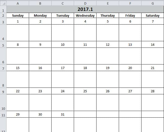

Você pode inserir algumas tarefas neste calendário. E a função é a mesma de um memorando. Ao utilizar o Excel, essas tarefas ficarão mais claras. Agora siga as etapas na parte seguinte e veja como funciona.

Criar um calendário

1. Pressione o botão “Alt +F11” no teclado para abrir a planilha.
2. E então insira um novo módulo no editor do Visual Basic.
3. Agora copiando os seguintes códigos para o novo módulo:

Sub Create_Monthly_Calender()
    Dim firstweekday As Integer, EndDay As Integer, _
    FirstWeekColumnIndex As Integer, AssignmentDate As Integer, _
    FirstCountNumber As Integer, SecondCountNumber As Integer, _
    LastDay As Range, objRange As Range, RowIndexofLastday As Integer, FirstCountforTargetRange As Integer, SecondCountforTargetRange As Integer

    firstday = InputBox("Input the year, month and the first day with this format: year/month/day")
    If firstday = "" Then Exit Sub


    Range("A1:G1").Merge
    Range("A1") = Year(firstday) & "." & Month(firstday)
    Range("A2") = "Sunday"
    Range("A2").AutoFill Destination:=Range("A2:G2"), Type:=xlFillDefault
    firstweekday = Application.WorksheetFunction.Weekday(firstday)
    Cells(3, firstweekday) = 1

    Select Case Month(firstday)
        Case 1, 3, 5, 7, 8, 10, 12
            EndDay = 31
        Case 4, 6, 9, 11
            EndDay = 30
        Case 2
            If (Year(firstday) Mod 4) = 0 And (Year(firstday) Mod 100) <> 0 Or ((Year(firstday) Mod 400) = 0) Then
                EndDay = 29
            Else
                EndDay = 28
            End If
    End Select

    For FirstWeekColumnIndex = 1 To (7 - firstweekday)
        Cells(3, firstweekday).Offset(0, FirstWeekColumnIndex) = Cells(3, firstweekday).Offset(0, FirstWeekColumnIndex - 1) + 1
    Next FirstWeekColumnIndex

    AssignmentDate = Range("G3") + 1
    For FirstCountNumber = 2 To 10 Step 2
        For SecondCountNumber = 0 To 6
            Cells(3, firstweekday).Offset(FirstCountNumber, 1 - firstweekday + SecondCountNumber) = AssignmentDate
            AssignmentDate = AssignmentDate + 1
            If Cells(3, firstweekday).Offset(FirstCountNumber, 1 - firstweekday + SecondCountNumber) = EndDay Then
                Exit For
            End If
        Next SecondCountNumber
        If Cells(3, firstweekday).Offset(FirstCountNumber, 1 - firstweekday + SecondCountNumber) = EndDay Then
            Exit For
        End If
    Next FirstCountNumber

    ’set format for the range
    With Range("A1")
        .HorizontalAlignment = xlCenter
        .VerticalAlignment = xlCenter
        .Font.Size = 16
        .Font.Bold = True
        .Interior.Color = RGB(196, 202, 201)
    End With

    With Range("A2:G2")
        .HorizontalAlignment = xlCenter
        .VerticalAlignment = xlCenter
        .Font.Bold = True
    End With

    For Each LastDay In ActiveSheet.UsedRange
        If LastDay = EndDay Then
            RowIndexofLastday = LastDay.Row
        End If
    Next

    For FirstCountforTargetRange = RowIndexofLastday To 3 Step -2
            With Range("A" & FirstCountforTargetRange, "G" & FirstCountforTargetRange)
                .HorizontalAlignment = xlCenter
                .VerticalAlignment = xlCenter
                .RowHeight = 20
            End With
    Next FirstCountforTargetRange

        For SecondCountforTargetRange = RowIndexofLastday + 1 To 4 Step -2
            With Range("A" & SecondCountforTargetRange, "G" & SecondCountforTargetRange)
                .HorizontalAlignment = xlCenter
                .VerticalAlignment = xlCenter
                .Font.Bold = True
                .RowHeight = 50
                .ColumnWidth = 12
            End With
    Next SecondCountforTargetRange

    Set objRange = Range("A1", "G" & (RowIndexofLastday + 1))
    With objRange.Borders
        .Color = vbBlack
        .Weight = xlThin
        .LineStyle = xlContinuous
    End With

    ActiveWindow.DisplayGridlines = False
    Cells(3, firstweekday).Offset(1, 0).Select
End Sub

Portanto, é uma macro muito solitária. Mas você pode usá-lo diretamente. E você não precisa modificá-lo.

4. Em seguida, pressione o botão “F5” no teclado.
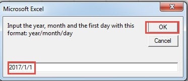
5. Na janela pop-up, insira a data do primeiro dia com o formato “Ano/Mês/Dia”. O “Dia” pode ser qualquer dia deste mês, aqui vamos inserir “1”.
6. E depois clique no botão “OK”. Em seguida, você voltará ao editor. Para verificar o resultado, você pode voltar para a planilha.

O calendário já apareceu na planilha. E o cursor será posicionado na célula em branco do primeiro dia.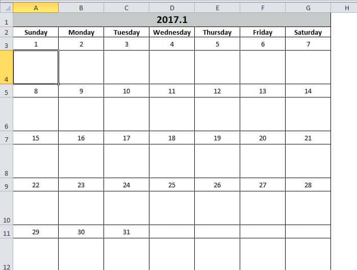

Por outro lado, se você não estiver satisfeito com o formato das células, também poderá modificar os códigos de acordo com sua preferência. Com este calendário, você certamente melhorará sua eficiência no trabalho.

O Excel não é menos propenso a falhas

Se você usa o Excel com frequência, não será difícil perceber que ele sempre acaba corrompendo. Na maioria das vezes, fechar e reiniciar o Excel resolve o problema. No entanto, às vezes você se depara com problemas graves de corrupção de dados. E nesse momento, você pode usar nossa poderosa ferramenta para... reparar erro de dados xlsx do ExcelUtilizando esta ferramenta, quase todos os erros podem ser resolvidos facilmente.

Introdução do autor:

Anna Ma é especialista em recuperação de dados em DataNumen, Inc., líder mundial em tecnologias de recuperação de dados, incluindo reparar arquivo docx do Word e produtos de software de reparo do Outlook. Para mais informações visite www.datanumen.com