Percentage is a very common data form in Excel. To make things easier, Excel has the feature of setting data to the percentage format.
There are 3 different methods to change the format. But you may also need to pay attention to some of the details. In this image below, we need to input the growth rates of sales volume manually.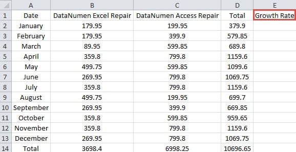
There are a lot of data that we need to input. Thus, if Excel can change the form into percentage format automatically, the task can be much easier.
Method 1: Use Shortcut Key Combo
The Shortcut key combo is very simple to use. Here the shortcut key combo is “Ctrl + Shift +%”. Actually, it is the same as clicking the button in the toolbar.
But using this combo before entering the number or after entering will produce different results. And we will discuss it in detail.
(1) Use after Entering the Number
- Input the number “0.12” into the target cell.
- Now press “Enter” or click another cell in the worksheet.
- And then click the cell again to position the cursor at the cell.
The above two steps will quit the edit mode. Otherwise the shortcut key cannot take effect. Here you may also notice that the cell category is “General”.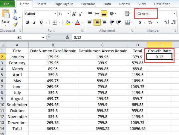
- Now press the keys “Ctrl + Shift +%” on the keyboard. And the percent sign will appear immediately. The number in the cell will become “12%”.
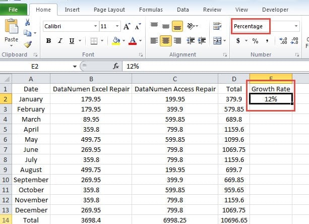
At this time, the cell category turns into “Percentage”. Therefore, if you need to use the shortcut combo after entering numbers, you need to divide the number by 100.
On the other hand, when it relates to decimals, things will be different. Excel will automatically round the number that you input into the cell.
The number will be multiplied by 100 after you use the shortcut keys. If there is no decimal point in the number, Excel will add the percent sign directly.
Otherwise, if first number after decimal point is greater than or equals to 5, the last number before decimal point will plus 1. Or it will not plus 1.
Thus, the result that appears in the cell will be whole number all the time. And you can check the original decimal form in the formula bar. If you still have difficulties about the rule, you may refer to some examples in the table below:
| The number you input | Use the shortcut key combo after entering the number. | The number multiplies 100 | Result in the cell | Result in the formula bar | Description |
| 2 | 200 | 200% | 200% | \ | |
| 0.54 | 54 | 54% | 54% | \ | |
| 0.543 | 54.3 | 54% | 54.3% | The first number after the decimal number is less than 5. | |
| 0.545 | 54.5 | 55% | 54.5% | The first number after the decimal number equals to 5. | |
| 0.0081 | 0.81 | 1% | 0.81% | The first number after the decimal number is greater than 5. | |
| 0.0021 | 0.21 | 0% | 0.21% | The first number after the decimal number is less than 5. |
(2) Use before Entering the Number.
- Click the cell. In this step, the cell category is still “General”.
- Now press “Ctrl + Shift +%”. After this action, the cell category will change into “Percentage”.
- And then input the number “12” into the cell. Excel will automatically add the percent sign after the number.
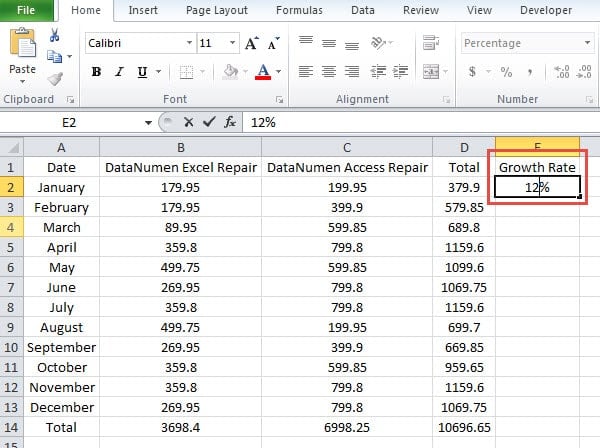
Hence, in this order, you don’t need to divide 100 before you enter the number.
In this order, Excel will also round the number if you enter a decimal number. Here the number that you enter will not multiply 100. Thus, if you enter a whole number, there will be no change. As for decimal number, the first number after decimal point is greater than or equals to 5, the last number before decimal point will plus 1. And it will not plus 1 if the number after decimal is less than 5. You can also refer to the table below for some examples.
| Use the shortcut keys before entering the number | The number you input | Result in the cell | Result in the formula bar | Description |
| 12 | 12% | 12% | \ | |
| 5.2 | 5% | 5.2% | The first number after the decimal number is less than 5. | |
| 5.8 | 6% | 5.8% | The first number after the decimal number is greater than 5. | |
| 0.81 | 1% | 0.81% | The first number after the decimal number is greater than 5. | |
| 0.23 | 0% | 0.23% | The first number after the decimal number is less than 5. |
The above are the differences of the order of using the shortcut combo. You can apply any of the two orders according to your need. In addition, you need to be more careful about the round feature in Excel.
(3) Disable the Automatic Percentage Entry
There is a feature of automatic percent entry in Excel.
- Click “File” in the ribbon.
- And then click “Options”.

- In the “Excel Options” window, click “Advanced”.
- And then uncheck the option “Enable automatic percentage entry”.
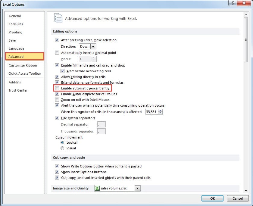
- Next, click “OK”. Now this feature has been disabled.
Now if you use the shortcut key combo after entering the number, you will get the same result as if this feature is still available.
But if you use the other order, the result will be different. The number that you input will also multiplies 100 before adding the percent sign. Besides, Excel will also round the number. Therefore, Excel will produce the same result as the order of using the shortcut key combo after entering the number.
Method 2: Change the Number Format in the Toolbar
In this method, you can change the number format in the toolbar.
(1) Change the Format before Entering the Number
- Enter the number 0.12 into the cell.
- Then click the small arrow of the number format.
- And then choose the option “Percentage” in the drop-down list. Thus, the format will change. The number you see in the cell will be 12.00%.
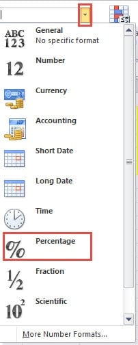
Here the number will multiply 100 and also add two decimal places to the number. If there are more than 2 decimals in the numbers that has multiplied 100, Excel will round the number.
If the third decimal is greater than or equals to 5, the second decimal will add 1. Otherwise, it will not add 1. You can refer to the table below:
| The number you input | Choose the option | The number that multiplies 100 | The result in cell | The result in the formula bar | Description |
| 12 | 1200 | 1200.00% | 1200.00% | \ | |
| 7.23 | 723 | 723.00% | 723.00% | \ | |
| 0.7234 | 72.34 | 72.34% | 72.34% | \ | |
| 0.72343 | 72.343 | 72.34% | 72.343% | The number of the third decimal is less than 5. | |
| 0.72345 | 72.345 | 72.35% | 72.345% | The number of the third decimal equals to 5. |
Besides, even if you uncheck the option “Enable automatic percentage entry”, you will get the same result.
(2) Change the Format after Entering the Number
Now you change the order, and here the number will not multiply 100. But as for the rule of rounding number, it also depends on the third decimal number. The table below also lists some of the examples.
| Choose the option | The number you input | The result in cell | The result in the formula bar | Description |
| 12 | 12.00% | 12.00% | \ | |
| 2.1 | 2.10% | 2.10% | \ | |
| 2.13 | 2.13% | 2.13% | \ | |
| 2.134 | 2.13% | 2.134% | The number of the third decimal is less than 5. | |
| 2.135 | 2.14% | 2.135% | The number of the third decimal equals to 5. |
Besides, if the option “Enable automatic percentage entry” is disables, you will get the same result as the order of changing the format before entering the number.
Method 3: Change the Cell Category in Format Cells
This method has some similarities with the previous one. But the place to change it is different.
Sentences below show the steps to change the category.
- First click the small arrow in the “Alignment” part.
- In the “Format Cell” window, check the tab “Number”.
- And then choose the option “Percentage”.
- And then set the decimal point in the “Decimal places”.
- After that, click “OK”. Thus, the cell category will change into “Percentage”.
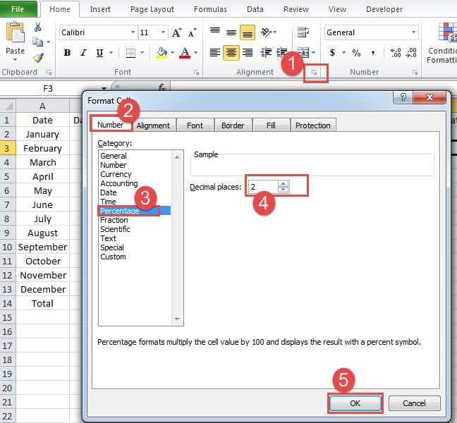
You can change the category before entering the number or after the entrance. Suppose the decimal place is 2, the result is exactly the same as change in the number format. This same result also includes the change of “Enable automatic percentage entry”. Besides, if the decimal place is different, such as 3, Excel will refer to the fourth number when rounding the number. Thus, you will know how the decimal place works here.
The above three methods will produce different results if you change the order or modify the option “Enable automatic percentage entry”. You can also have a try and use the most suitable method in your worksheet.
Do Not Panic when Excel corrupts
Sometimes you will meet with Excel file corruption. At this moment, don’t panic. The actions that you do at the beginning of the will determine whether the file can survive. You can contact our Excel experts immediately and get the Excel fix tool to repair Excel. If you try to repair it by yourself without figuring out the reason, no one can guarantee the result.
Author Introduction:
Anna Ma is a data recovery expert in DataNumen, Inc., which is the world leader in data recovery technologies, including word recovery and outlook repair software products. For more information visit www.datanumen.com

Leave a Reply